Artificial Intelligence is on the front page of all newspapers those days (often for the wrong reasons…). Of course, AI is not new, the field dating from the middle of last century; neither are cascading neural networks, which I used in the 1990s to predict protein’s secondary structures. However, it really exploded with Deep Learning. Some stories made the news over the years, for instance, DeepMind’s AlphaGo beating a Go’s world champion and AlphaFold solving the long-standing problem of predicting protein’s 3D structures (well, at least the non-flexible conserved parts…). Still, most successes remained confined to their respective domains (e.g., environment recognition for autonomous vehicles, tumour identification and machine translation such as Google Translate and DeepL). However, what brought AI to everyone’s attention was OpenAI’s DALL’E and, more recently, ChatGPT, which can generate images and text following a textual prompt.
OpenAI actually developed many other Deep Learning models, some open source. Among those, Whisper models promise to be a real improvement in speech recognition and transcription. Therefore, I decided to test Whisper on two different tasks: a scientific presentation containing technical terminology, given by a US speaker, and a song containing cultural references, sung by an American singer but with no accent (i.e., BBC-like…).
Lenovo Thinkpad T470 I, no GPU. Linux Ubuntu 22.10 Python 3.10.7 Pytorch 2.0 I used the model for speech recognition in the video editing tool Kdenlive 23.04 (Update 31 May 2023: I was able to run Whisper on Linux Ubuntu 23.04 with Python 3.11.2 and Kdenlive 23.04.1 ; although installing all the bits and pieces was not easy)
Whisper can be used locally or through an API via Python or R (for instance with the package openai), although a subscription might be needed if you already used all your free tokens.
There are five Whisper models.
Models
Parameters
Required VRAM
Relative speed
Tiny
39 M
~1 GB
~32x
Base
74 M
~1 GB
~16x
Small
244 M
~2 GB
~6x
Medium
769 M
~5 GB
~2x
Large
1550 M
~10 GB
1x
Note that these models run perfectly well on CPUs. While GPUs are necessary for training Deep Learning models, this is not the case when using them (although running them on CPU will always be slower because of floating point computations).
As an external “control”, I used the VOSK model vosk-model-en-us-0.22 (just called VOSK in the rest of this text).
NB: this is an anecdotal account of my experience, and does not replace comprehensive and systematic tests, for instance, using datasets such as Tedlium. or LibriSpeech test-clean
I used speech recognition to create subtitles, as it represents the final aim in 95% of my professional transcriptions. Many videos are available to explain how to generate subtitles in Kdenlive, including with Whisper.
Transcription of a scientific presentation
The first thing I observed was the split into text fragments. I noticed that their placement along the timeline (the timecodes) was systematically off, starting and finishing too early. Since this did not depend on the model, the problem could come from Kdenlive.
The length of the text fragments varied widely. VOSK produced small fragments, perfect for subtitles, but cut anywhere. Indeed, VOSK does not introduce punctuation and has no notion of sentence. The best fragments were provided by Tiny and Large. They were small, perfect for subtitles, and cut at the right places. On the contrary, Small produced fragments of consistent lengths, longer than Tiny and Large, and thus too long for subtitles, while the fragments produced by Base and Medium were very heterogeneous, only cut after periods.
The models differed straight from the beginning. Tiny produced text that was much worse than VOSK (if we ignore the absence of punctuation by the latter). “professor at pathology” instead of “of pathology”, a missing “and”, a period replaced by a comma, and a quite funny “point of care testing” transformed into “point of fear testing”! All the other models produced perfect texts, Small, Medium, and Large even adhering to my beloved Oxford comma.
VOSK: welcome today i'm john smith i'm a professor of pathology microbiology and immunology and medical director of clinical chemistry and point of care testing
Tiny: Welcome today, I'm John Smith. I'm a professor at Pathology, Microbiology, Immunology, and Medical Director of Clinical Chemistry and Point of Fear Testing.
Base: Welcome today. I'm John Smith. I'm a professor of pathology, microbiology and immunology and medical director of clinical chemistry and point of care testing.
Small: Welcome today. I'm John Smith. I'm a professor of pathology, microbiology, and immunology, and medical director of clinical chemistry and point of care testing.
Medium: Welcome today. I'm John Smith. I'm a professor of pathology, microbiology, and immunology and medical director of clinical chemistry and point of care testing.
Large: Welcome today. I’m John Smith. I'm a professor of pathology, microbiology, and immunology, and medical director of clinical chemistry and point of care testing.
A bit further, the speaker described blood gas analysers. VOSK can only analyse speech using dictionaries. As such, it could not guess that pH, pCO2, and pO2 represent acidity, partial pressure of carbon dioxide and partial pressure of oxygen, respectively and spell them correctly. It also missed the p in pCO2. The result is still understandable for a specialist but would give odd subtitles.. The Whisper models consider the whole context, and can thus infer the correct meaning of the words. Tiny did not understand pH and pCO2, merging them. All the other models produced perfect texts.
VOSK: [...] instruments came out for p h p c o two and p o two
Tiny: [...] instruments came out for PHPCO2 and PO2.
Base: [...] instruments came out for pH, PCO2 and PO2
Small: [...] instruments came out for PH, PCO2, and PO2.
Medium: [...] instruments came out for pH, PCO2, and PO2.
Large: [...] instruments came out for pH, PCO2, and PO2.
VOSK’s dictionaries sometimes gave it an edge. For instance, it knew that co oximetry was a thing, albeit missing a dash. Only Large got it right here, Base, and Medium hearing coaximetry, and Tiny even hearing co-acemetery!
VOSK: [...] we saw co oximetry system
Tiny: [...] we saw co-acemetery systems.
Base: [...] we saw coaximetry systems.
Small: [...] we saw coaxymetry systems.
Medium: [...] we saw coaximetry systems.
Large: [...] we saw co-oxymetry systems.
Another example is the name of chemicals. VOSK recognised benzalkonium, which was recognised only by Medium. Interestingly, the worst performers were Base, which misheard benzylconium, and Large, which misheard benzoalconium (Tiny and Small heard properly but spelt the word wrong, with a ‘c’ instead of a ‘k’).
The way Whisper Large can understand mispronounced words is very impressive. In the following example, Small and Large are the only models correctly recognising that there are two separate sentences. More importantly, VOSK and Tiny could not identify the word “micro-clots”. The hyphenation is a matter of discussion. While the parsimonious rule should apply (do not use hyphens except when not doing so would generate pronunciation errors), using hyphens after micro and macro are commonplace.
VOSK: [...] to correct the problem like micro plots and and i discussed the injection of a clot busting solution
Tiny: […] to correct the proper microplasks. And I discussed the injection of a clock-busting solution.
Base: […] to correct the problem like microclots and I discussed the injection of a clot busting solution.  (wrong start)
Small: […] to correct the problem, like microclots. And I discussed the injection of a clot-busting solution.
Medium: […] to correct the problem, like microclots, and I discussed the injection of a (wrong start, missed end of sentence.)
Large: […] to correct the problem, like micro-clots. And I discussed the injection of a clot-busting solution.
In conclusion, Whisper Large is the best model, not surprisingly, with the surprising exception of the small mistake on “benzalkonium”.
Transcription of a pop culture song
Adding sound on top of speech, such as music, can throw off speech recognition systems. Therefore, I decided to test the models on a song. I chose a very simple song with slow and clearly enunciated lyrics. And frankly, being a nerd, I relished highlighting those fantastic Wizard Rock scene artists whose dozen groups have been celebrating the Harry Potter universe through hundreds of great songs. I used a song from Tonks and the Aurors entitled “what does it means”.
The first massive observation was that I could not compare VOSK to Whisper models. Indeed, the former is absolutely unable to recognise anything. The “transcription” was made of 27 small fragments of complete gibberish, with barely a few correct words. Only one fragment contained an actual piece of the lyrics: “Everybody says that it’s probably nothing”. However, these words were also identified by all Whisper models.
Now for the Whisper models. The overall recognition was remarkable. On the front of fragment size, only Tiny produced small fragments, perfect for subtitles, cut at the right places. Medium was not too bad. Base and Small produced heterogeneous fragments, only cut after periods. Large produced super short segments, often made up of one word. Initially, I thought this was very bad. However, I then realised that it was perfect for subtitling the song; just the right rate in character per second, very readable.
Something odd happened at the start, with some models adding fragments while there was no speech, such as “Add text” (Tiny) or “Music” (Base). Large added the Unicode character “♪” whenever they were music and no speech, which I found nice.
When it came to recognise characters from Harry Potter, the models performed very differently. Tiny and Base did not recognise Mad-Eye Moody. And they also failed to distinguish between Mad-Eye and Molly (Weasley). They also made several other mistakes, e.g. “say” instead of “stay”. Tiny even mistook “vigilant” for “vigilance” and completely ignored the word “here”. It also interpreted “sympathy” in the rather bizarre, “said, but me”!
Tiny: Dear, Maddie, I'm trying to say constantly vigilance
Base: Dear, Madhy, I'm trying to say, Constantly vigilant Here,
Small: Dear Mad Eye, I'm trying to stay constantly vigilant Here,
Medium: Dear Mad-Eye, I'm trying to stay constantly vigilant here
Large: Dear mad eye I'm trying to stay constantly vigilant Here
Tiny: Dear, Maddie, thanks a lot for your tea and said, but me
Base: Dear, Madhy, thanks a lot for your tea and sympathy
Small: Oh, dear Molly, thanks a lot for your tea and sympathy (“Oh” should be on a segment of its own)
Medium: Oh, dear Molly, thanks a lot for your tea and sympathy (“Oh” should be on a segment of its own)
Large: Dear Molly Thanks a lot for your tea and sympathy
Another example of context-specific knowledge is the Patronus. Note that such a concept is absolutely out of reach for models using dictionaries. Only machine learning models trained with Harry Potter material can work it out. And this is the case for Medium and Large. Small is not so far, while Tiny and Base try to fit the sounds into a common word.
Tiny: But I can't stop thinking about my patrolness
Base: but I can't stop thinking about my patrolness
Small: Here, but I can't stop thinking about my Patronas
Medium: But I can't stop thinking about my Patronus
Large: But I Can't stop Thinking about My Patronus
Tiny and Base also made several other errors, mistaking “phase” for “face”, or “starlight” for “start light”.
Interestingly, Tiny hallucinated 40 seconds of “Oh, oh, oh, oh” at the end of the the song, while Base, Small, and Medium hallucinated a “Thank you for watching”.
Conclusion
While Medium provided an overall slightly better text, Large provided the best subtitles for the song, without hallucinations.
Overall, for both task Open AI WhisperLarge provided an excellent job, surpassing many human transcriptions I had to deal with, in particular when it comes to technical and non-standard terms.
COVID-19 pandemics put mathematical models of biological relevance all over daily newspapers and TV news, raising their profile for the non-scientists. In the life sciences, while mathematical models have always been at the core of some disciplines, such as genetics, they really became mainstream with the rebirth of systems biology a couple of decades ago. However, there are many different modelling approaches, and even specialists often ignore methods they do not use regularly or have not been taught.
After a historical overview, this blog post will then attempt to classify the main types of models used in systems biology according to their principal modalities.
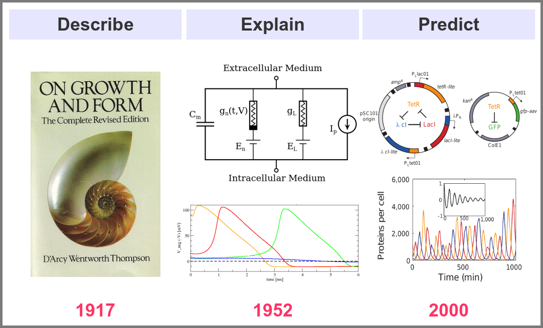
What is the goal of using mathematical models in the life sciences in the first place? Three main aims came out roughly sequentially during the XX century, following the path physics followed over the past two millennia. First, mathematics helps describe the structure and dynamics of living forms and their productions. These models may rely on supposed underlying laws, be purely descriptives, such as the allometric laws. A great example is the famous book “On Growth and Form” by D’Arcy Thompson, attempting to understand living forms based on physical laws.
The second aim is to explain the shape and function of living forms. How do the properties of life’s building blocks explain what we can observe? In their masterwork, Alan Hodgkin and Andrew Huxley predicted the existence of ionic channels within the cell membrane and, using a mathematical model, explained how neurons generate action potentials (a work for which they got the Nobel prize).
Finally, can we predict how a system will behave, and can we invent new systems that will behave the way we want them to? This is the purpose of synthetic biology, exemplified in the figure below by the pioneering work of Michael Elowitz and Stanislas Leibler, who built the “repressilator”, a synthetic construct exhibiting sustained oscillations maintained through generations of bacteria.
Obviously, there are no strict boundaries between the three aims, and most models seek to describe, explain, and predict the structures and behaviours of living systems.
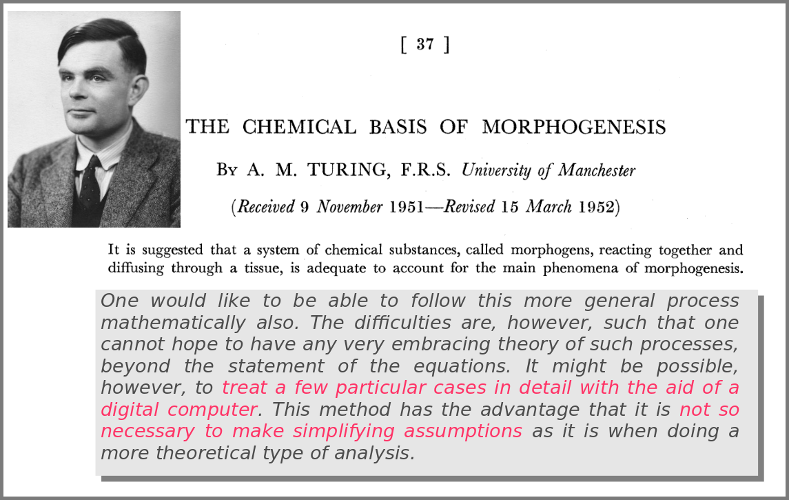
A major shift in the use of mathematical models was the introduction of numerical simulations, made feasible by the invention of computers. The benefits have been laid out by one of the inventors of such computers in an article that indeed contained complex mathematical models but no simulations. In his famous 1952 paper introducing morphogens, Alan Turing suggested that using a digital computer to simulate specific cases of a biological system would allow avoiding the oversimplifications required by analytic solutions.
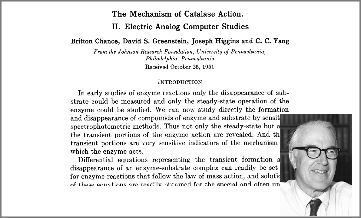
This wish was granted the very same year first by Britton Chance, who built a computer (an analogue one at the time) specifically to solve a differential equation model of a small biochemical pathway.
1952 was also when Hodgkin and Huxley published the action potential model mentioned above, a real Annus Mirabilis for computational modelling in the life sciences.
Before going further, we should ask ourselves, “what is a mathematical model”? According to Wikipedia (as of 4th July 2022), Amathematical model is a description of a system using mathematical concepts and language. I consider that three essential categories of components form mathematical models in systems biology.
Variables represent what we want to know or what we want to compare with the observations. They can characterise a physical entity, e.g., the concentration of a substance, the length of an object or the duration of an event, or be derived from the model itself, for instance, the maximum velocity of an enzymatic reaction.
Relationships mathematically link variables together and represent what we know or what we want to test. They can be static, an affinity constant linked to concentrations or dynamic, such as a rate of change depending on concentrations. Relationships are not necessarily equations. For instance, a sampling might link a variable to a statistical distribution, and logic models use logical statements to attribute values to variables.
Finally, a much-underestimated category is formed by constraints put on the model. Those represent the context of the modelling project or what we consciously decide to ignore. Some constraints are properties of the world, e.g., a concentration must always be positive, the total energy is conserved, and some are properties of the model, such as boundary conditions and objective functions for optimisation procedures. Initial conditions – the values of variables before starting a numerical simulation – are also crucial since a given model might behave differently with different initial conditions, even if neither variables nor relationships are changed.
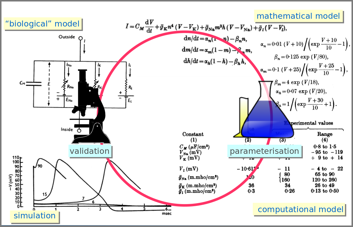
However, the mathematical model itself is only one brick of a systems biology’s modelling and simulation project as in any natural science domain. Since these models aim to be mechanistic, i.e., anchored in underlying molecular, cellular, tissular, and physiological processes, the first step is to conceptualise a “biological model”. For instance, a biochemical pathway will be a collection of chemical reactions. In the case of Hodgkin and Huxley, who did not know the underlying molecules, the mechanism was based on an electrical analogy, ionic channels being represented by electrical conductances. The “mathematical model” is made up of mathematical relationships linking the variables and constraints. A “computational model”, using the “mathematical model” in conjunction with observed or estimated values, is then simulated. The result is compared with observations, and the loop is iterated.
Now let’s explore the different facets of models used in systems biology, and marvel at their diversity
The variables of a model can represent biological reality at different granularities. In some logical models (often wrongly called Boolean networks), a variable can represent a state, such as presence or absence, 1, 2, 3. Detailed models at the “mesoscopic scale” might represent individual molecules, where a separate variable represents every single particle. Variables can also represent discrete populations of molecules, for instance, the number of molecules of a given chemical class, whose evolution is simulated by stochastic algorithms. In chemical kinetics, the variables whose change is determined using ordinary differential equations often represent continuous concentrations. Finally, some models gloss over the physical parts altogether and use fields to represent what could happen to them.
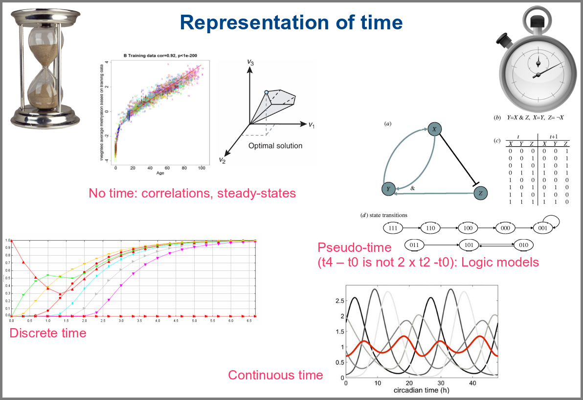
Numerical simulations most often represent the evolution of variable values over “time”. However, the granularity of this “time” may vary. At an extreme, we have models with no representation of time, such as regression models, or implicit representation of time, such as steady-states models. In logical models, as in Petri Net, simulations usually progress along a pseudo-time, where one cannot compare numbers of steps. Time can be discrete, numerical simulations computing a system’s state at fixed intervals, for instance, one second. Finally, models can consider time as continuous, simulations being iterated at various timepoints decided by numerical solvers (note that software might still return results at fixed intervals).
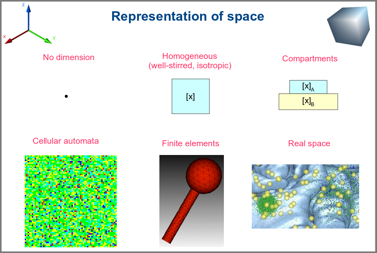
Spacetime being a thing, we also have as many different representations of space. Starting with no space at all, for instance, in noncompartmental analyses of pharmacokinetic models. Space can also be represented by a single homogenous (well-stirred) and isotropic compartment or several of them connected by variables and relationships (multi-compartment models, a.k.a. bathtub models). Cellular automata constitute a particular case, where each compartment is also a model variable whose status depends on its neighbours’. An extension of the multi-compartment modelling represents realistic biological structures using finite elements, each considered homogeneous and isotropic. Finally, space might be represented by continuous variables, where the trajectory of each molecule can be simulated.
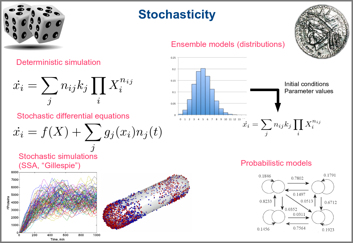
Variability and noise are unavoidable parts of any observation of the natural world, including living systems. Variability can be extrinsic (e.g., due to technical variability), or intrinsic (e.g., actual differences between cells or samples). True noise depends on the size of the system. Taking all those into account in the models can thus be important, and different approaches present different levels and types of stochasticity. As with the other modalities above, stochasticity might be entirely absent, models and simulations being deterministic. One can add different and arbitrary types of noise to simulations with stochastic differential equations. The stochastic aspect might instead emerge directly from the structure of the model, as with the Stochastic Simulation Algorithms (a.k.a. algorithms of the “Gillespie” type). Variability can also be taken into account prior to the simulations, for instance, by sampling initial conditions from distributions, as with ensemble modelling. Finally, in probabilistic models such as Markov models, the entire iteration of the system is based on the probabilities of switching states.
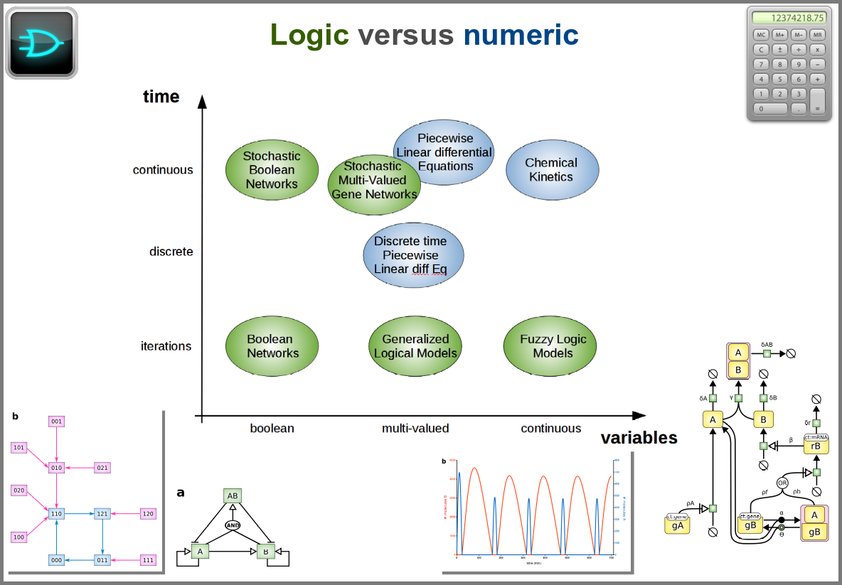
Finally, there are two large families of models based on the type of algorithms used to update the variables. One can compute a variable’s new value by calculating its value either using numerical combinations of previous variables’ values or logic rules taking into account other variable states. Contrary to widespread belief, not all logic models use pseudo-time and Boolean variables. Stochastic Boolean networks can use continuous time, and fuzzy logic models can base their decision on continuous variable values.
Those modalities can be combined in many ways to produce an extremely rich toolkit of modelling approaches. One of the most frequent sources of pain when modelling biological systems is to start with a methodological a priori, often because we are comfortable with an approach, we have the necessary software, or we don’t know better. Doing so can result in under-determined models, endless iterations and failure to get any result. The choice of a modelling approach should be first and foremost based on: 1) the question asked, and 2) the data available to build and validate the model.
References
Chance, B., Greenstein, D. S., Higgins, J. & Yang, C. C. (1952) The mechanism of catalase action. II. Electric analog computer studies. Arch. Biochem. Biophys.37: 322–339. doi:10.1016/0003-9861(52)90195-1
Hodgkin, A.L., Huxley, A.F. (1952). A quantitative description of membrane current and its application to conduction and excitation in nerve. The Journal of Physiology. 117 (4): 500–44. doi:10.1113/jphysiol.1952.sp004764
Stanislas Leibler; Elowitz, Michael B. (2000-01-20). “A synthetic oscillatory network of transcriptional regulators”. Nature403 (6767): 335–338. doi:10.1038/35002125.
Thompson, D. W., 1917. On Growth and Form. Cambridge University Press.
Turing, A. M. (1952). “The chemical basis of morphogenesis”. Philosophical Transactions of the Royal Society of London B. 237 (641): 37–72. doi:10.1098/rstb.1952.0012.
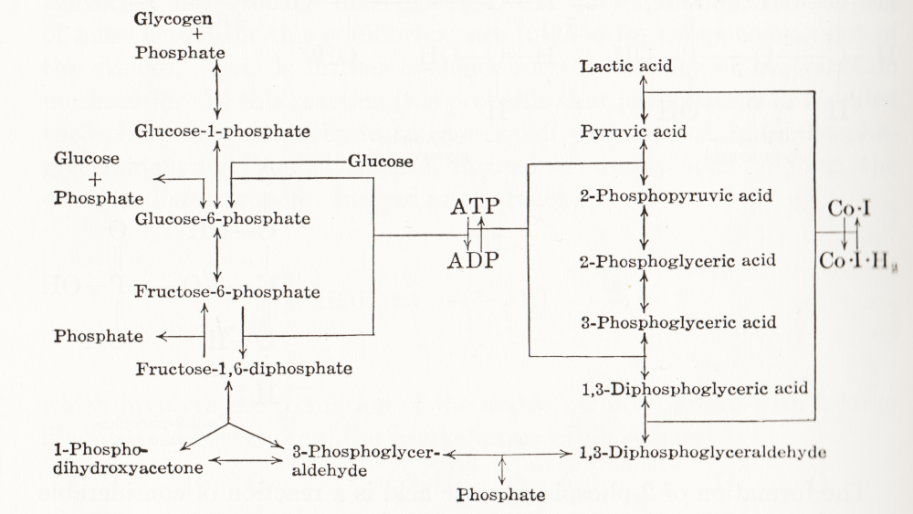
Visual representation of biochemical pathways has been a critical tool for understanding the cellular and molecular systems for a long time. Any knowledge integration project involves a jigsaw puzzle step, where different pieces must be put together. When Feynman cheekily wrote on his blackboard just before his death, “What I cannot create I do not understand”, he meant that he only fully understood a system once he derived a (mathematical) model for it; and interestingly, Feynman is also famous for one of the earliest standard graphical representations of reaction networks, namely the Feynman diagrams to represent models of subatomic particle interactions. The earliest metabolic “map” I possess comes from the 3rd edition of “Outlines of Biochemistry” by Gortner published in 1949. I would be happy to hear if you have older ones.
(I let you find out all the inconsistencies, confusing bits, and error-generating features in this map. This might be food for another text, but I believe this to be a great example to support the creation of standards, best practices, and software tools!)
Until recently, those diagrams were drawn mainly by hand, initially on paper, then using drawing software. There was little thought spent on consistency, visual semantics, or interoperability. This state of affairs changed in the 1990s as part of Systems Biology’s revival. The other thing that changed in the 1990s was the widespread use of computers and software tools to build and analyse models. The child of both trends was the development of standard computer-readable formats to represent biological networks.
When drawing a knowledge representation map, one can divide the decision-making process, and therefore the things we need to encode in order to share the map, into three parts:
What – How can people identify what I represent? A biochemical map is a network built up from nodes linked by arcs. The network may contain only one type of node, for instance, a protein-protein interaction network or an influence network, or be a bipartite graph, like a reaction network – one type of node representing the pools involved in the reactions, the other representing the reactions themselves. One decision is the shape to use for each node so that it carries visual information about the nature of what it represents. Another concerns the arcs linking the nodes, which can also contain visual clues, such as directionality, sign, type of influence, and more. All this must be encoded in some way, either semantically (a code identifying the type of glyphs from an agreed-up list of codes) or graphical (embedding an image or describing the node).
Where – After choosing the glyphs, one needs to place them. The relative position of the information should not always carry much information, but there are some cases where it must, e.g. members of complexes, inclusion in compartments, etc. Furthermore, there is no denying that the relative position of glyphs is also used to convey more subjective information. For instance, a linear chain of reactions induces the idea of a flow, much better than a set of reactions going randomly up and down, right and left. Another unwritten convention is to represent membrane signal transduction on the top of the maps, with the “end-result” – often effect on gene expression – at the bottom, with the idea of a cascading flux of information. The coordinates of the glyphs must then be shared as well.
How – Finally, the impact of a visual representation also depends on aesthetic factors. The relative size of glyphs and labels, the thickness of arcs, the colours, shades and textures, all influence the facility with which viewers absorb the information contained in a map. Relying on such aspects to interpret the meaning of a map should be avoided, particularly if the map is to be shared between different media, where rendering could affect the final aspect. Nevertheless, wanting to keep this aspect as close as possible makes sense.
A bit of history
Different formats have been developed over the years to cover these different aspects with different accuracy and constraints. In order to understand why we have such a variety of description formats on offer, a bit of history might be helpful. Being able to encode the graphical representation of models in SBML was mentioned as early as 2000 (Andrew Finney. Possible Extensions to the Systems Biology Markup Language. 27 November 2000).
In 2002, the group of Hiroaki Kitano presented a graphical editor for the Systems Biology Markup Language (SBML, Hucka et al 2003, Keating et al 2020), called SBedit, and proposed extensions to SBML necessary for encoding maps (Tanimura et al. Proposal for SBEdit’s extension of SBML-Level-1. 8 July 2002). This software later became CellDesigner (Funahashi et al 2003), a full-featured modelling developing environment using SBML as its native format. All graphical information is encoded in CellDesigner-specific annotations using the SBML extension system. In addition to the layout (the where), CellDesigner proposed a set of standardised glyphs to use for representing different types of molecular entities and different relationships (the what) (Kitano et al 2003). At the same time, Herbert Sauro developed an extension to SBML to encode the maps designed in the software JDesigner (Herbert Sauro. JDesigner SBMLAnnotation. 8 January 2003). Both CellDesigner and JDesigner annotations could also encode the appearance of glyphs (the how).
Once the SBML Layout annotations were finalised, the SBML and BioPAX communities came together to standardise visual representations for biochemical pathways. This led to the Systems Biology Graphical Notation, a set of three standard graphical languages with agreed-upon symbols and rules to assemble them (the what, Le Novère et al 2009). While the shape of SBGN glyphs determines their meaning, neither their placement in the map nor their graphical attributes (colour, texture, edge thickness, the how) affect the map semantics. SBGN maps are ultimately images and can be exchanged as such, either in bitmaps or vector graphics. They are also graphs and can be exchanged using graph formats like GraphML. However, sharing and editing SBGN maps would be much easier if more semantics were encoded than graphical details. This feeling led to the development of SBGN-ML (van Iersel et al 2012), which encodes not only the SBGN part of SBGN maps but also the layout and size of graph elements.
So we have at least three solutions to encode biochemical maps using XML standards from the COMBINE community (Hucka et al 2015):
1) SBGN-ML,
2) SBML with Layout extension (controlled Layout annotations in Level 2 and Layout package in Level 3), and
3) SBML with proprietary extensions.
Regarding the latter, we will only consider the CellDesigner variant for two reasons. Firstly, CellDesigner is the most used graphical model designer in systems biology (at the time of writing, the articles describing the software have been cited over 1000 times). Secondly, CellDesigner’s SBML extensions are used in other software tools. These three solutions are not equivalent; they present different advantages and disadvantages, and round-tripping is generally impossible.
SBGN-ML
Curiously, despite its name, SBGN-ML does not explicitly describe the SBGN part of the maps (the what). Since the shape of nodes is a standard, it is only necessary to mention their type, and any supporting software will know which symbol to use. For instance, SBGN-ML will not specify that a protein X must be represented with a round-corner rectangle. It will only say that there is a macromolecule X at a particular position with given width and height. Any SBGN-supporting software must know that a round-corner rectangle represents a macromolecule. The consequence is that SBGN-ML cannot be used to encode maps using non-SBGN symbols. However, software tools can decide to use different symbols attributed to a given class of SBGN objects while rendering the maps. For example, instead of using a round-corner rectangle each time a glyph’s class is macromolecule, it could use a star. The resulting image would not be an SBGN map. However, if modified and saved back in SBGN-ML, it could be recognised by another supporting software. Such behaviour is not to be encouraged if we want people to get used to SBGN symbols, but it provides a certain level of interoperability.
What SBGN-ML explicitly describes instead are the parts that SBGN itself does not regulate but are specific to the map. That includes the size of the glyphs (bounding box), the textual labels, as well as the positions of glyphs (the where). SBGN-ML currently does not encode rendering properties such as text size, colours and textures (the how). However, the language provides an element extension, analogous to the SBML annotation, that allows augmenting the language. One can use this element to extend each glyph or encode style, and the community started to do so in an agreed-upon manner.
Note that SBGN-ML only encodes the graph. While it contains a certain amount of biological semantics – linked to the identity of the glyphs – it is not a general-purpose format that would encode advanced semantics of regulatory features such as BioPAX (Demir et al. 2010), or mathematical relationships such as SBML. However, users can distribute SBML files along with SBGN-ML files, for instance, in a COMBINE Archive (Bergmann et al 2014). Unfortunately, there is currently no blessed way to map an SBML element, such as a particular species, to a given SBGN-ML glyph.
SBML Level 3 + Layout and Render packages
As we mentioned before, SBML Level 3 provides two packages helping with the visual representations of networks: Layout (the where) and Render (the how). Contrarily to SBGN-ML, which is meant to describe maps in a standard graphical notation, the SBML Level 3 packages do not restrict the way one represents biochemical networks. This provides more flexibility to the user but decreases the “stand-alone” semantics content of the representations. I.e. if non-standard symbols are used, their meaning must be defined in an external legend. It is, of course, possible to use only SBGN glyphs to encode maps. The visual rendering of such a file will be SBGN, but the automatic analysis of the underlying format will be more challenging.
The SBML Layout package permits encoding the position of objects, points, curves and bounding boxes. Curves can have complex shapes encoded as Béziers curves. The package allows distinguishing between different general types of nodes such as compartments, molecular species, reactions and text. However, there is little biological semantics encoded by the shapes, either regarding the nodes (e.g. nothing distinguishes a simple chemical from a protein) or the edges (one cannot distinguish an inhibition from a stimulation). In addition, the SBML Render package permits to define styles that can be applied to types of glyphs. This includes colours and gradients, geometric shapes, properties of text, lines, line-endings etc. Render can encode a wide variety of graphical properties, and pave the gap to generic graphical formats such as SVG.
If we are trying to visualise a model, one advantage of using SBML packages is that all the information is included in a single file, providing a straightforward mapping between the model constructs and their representation. This goes a long way to solve the issue of the biological semantics mentioned above since it can be retrieved from the SBML Core elements linked to the Layout elements. Let us note that while SBML Layout+Render do not encode the nature of the objects represented by the glyphs (the what) using specific structures, this can be retrieved via the attributes sboTerm of the corresponding SBML Core elements, using the appropriate values from the Systems Biology Ontology (Courtot et al 2011).
CellDesigner notation
CellDesigner uses SBML (currently Level 2) as its native language. However, it extended it with its own proprietary annotation, keeping the SBML perfectly valid (which is also the way software tools such as JDesigner operate). Visually, the CellDesigner notation is close to SBGN Process Descriptions, having been the strongest inspiration for the community effort. CellDesigner offers an SBGN-View mode, that produces graphs closer to pure SBGN PD.
CellDesigner’s SBML extensions increase the semantics of SBML elements such as molecular species or regulatory arcs in a way not dissimilar to SBGN-ML. In addition, it provides a description of each glyph linked to the SBML elements, covering the ground of SBML Layout and Render. The SBML extensions being specific to CellDesigner, they do not offer the flexibility of SBML Render. However, the limited spectrum of possibilities might make the support easier.
CellDesigner notation
SBML Layout+Render
SBGN-ML
Encodes the what
✓
✓
✓
Encodes the where
✓
✓
✓
Encodes the how
✓
✓
✓
Contains the mathematical model part
✓
✓
✗
Writing supported by more than 1 tool
✗
✓
✓
Reading supported by more than 1 tool
✓
✓
✓
Is a community standard
✗
✓
✓
Examples of usages and conversions
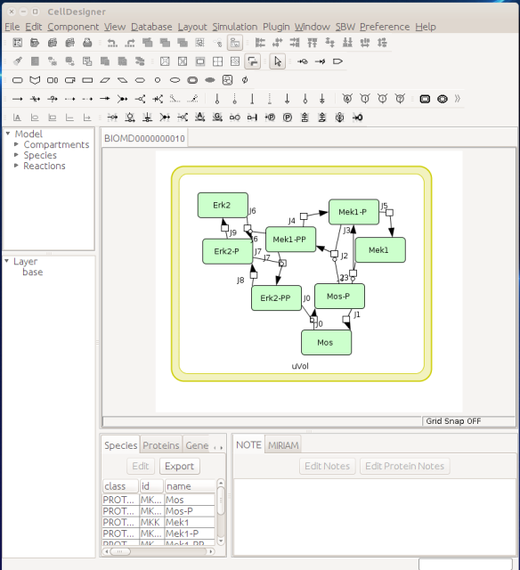
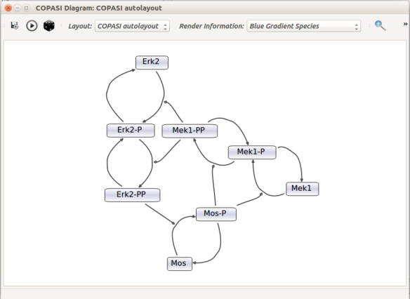
Now let us see the three formats in action. We start with SBGN-ML. First, we can load a model – for instance from BioModels (Chelliah et al 2015 ) – in CellDesigner (version 4.4 at the time of writing). Here we will use the model BIOMD0000000010, an SBML version of the MAP kinase model described in Kholodenko et al (2000).
From an SBML file that does not contain any visual representation, CellDesigner created one using its auto-layout functions. One can then export an SBGN-ML file. This SBGN-ML file can be imported, for instance, in Cytoscape (Shannon et al. 2003) 2.8 using the CySBGN plugin (Gonçalves et al 2013).
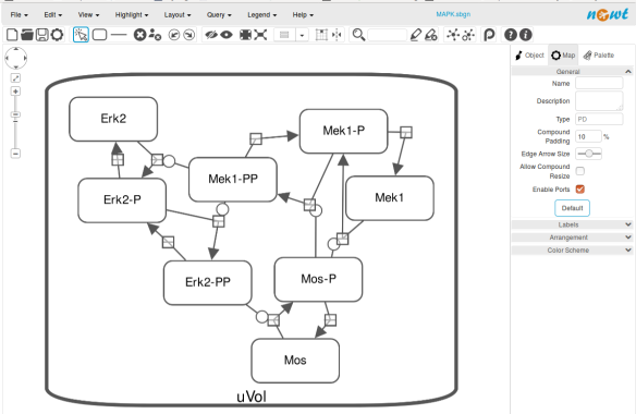
The position and size of nodes are conserved, but edges have different sizes (and the catalysis glyph is wrong). The same SBGN-ML file can be open in the online SBGN editor Newt.
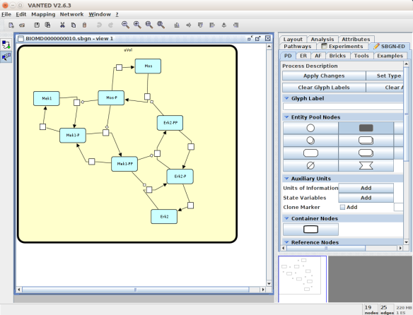
An alternative to CellDesigner to produce the SBGN-ML map could be Vanted (Junker et al 2006, version 2.6.4 at the time of writing). Using the same model from BioModels, we can auto-layout the map (we used the organic layout here) and then convert the graph to SBGN using the SBGN-ED plugin (Czauderna et al 2010).
The map can then be saved as SBGN-ML and as before, opened in Newt.
The positions of the nodes are conserved. However, the connection of edges is a bit different. In that case, Newt is slightly more SBGN compliant.
Then, let us start with a vanilla SBML file. We can import our BIOMD0000000010 model in COPASI (Hoops et al 2006, version 4.22 at the time of writing). COPASI now offers auto-layout capabilities, with the possibility of manually editing the resulting maps.
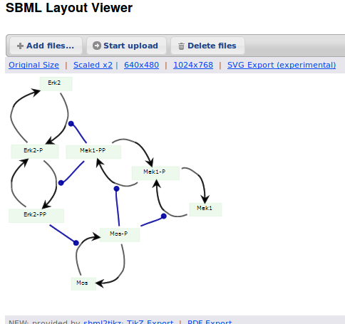
When we export the model in SBML, it will now contain the map encoded with the Layout and Render packages. When the model is uploaded in any software tool supporting the packages, we will retrieve the map. For instance, we can use the SBML Layout Viewer. Note that if the layout is conserved, it is not the case with the rendering.
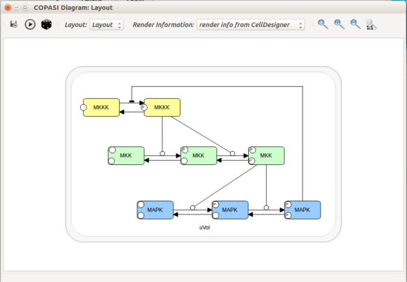
Alternatively, we can load the model to CellDesigner, and manually generate a nice map (NB: a CellDesigner plugin that can read SBML Layout was implemented during Google Summer of Code 2014 . It is part of the JSBML project).
We can create an SBML Layout using the CellDesigner layout converter. Then, when we import the model in COPASI, we can visualise the map encoded in Layout. NB: here, the difference in appearance is due to a problem in the CellDesigner converter, not COPASI.
The same model can be loaded in the SBML Layout Viewer.
How do I choose between the formats?
There is, unfortunately, no unique solution at the moment. The main question one has to ask is what do we want to do with the visual maps?
Are they meant to be a visual representation of an underlying model, the model being the critical part that needs to be exchanged? If that is the case, SBML packages or CellDesigner notation should be used.
Does the project mostly/only involves graphical representations, and those must be exchanged? CellDesigner or SBGN-ML would therefore be better.
Does the rendering of graphical elements matter? In that case, SBML packages or CellDesigner notations are currently better (but that is going to change soon).
Is standardisation important for the project, in addition to immediate interoperability? If yes, SBML packages or SBGN-ML would be the way to go.
All those questions and more have to be clearly spelt out at the beginning of a project. The answer will quickly emerge from the answers.
Acknowledgements
Thanks to Frank Bergmann, Andreas Dräger, Akira Funahashi, Sarah Keating, Herbert Sauro for help and corrections.
References
Bergmann FT, Adams R, Moodie S, Cooper J, Glont M, Golebiewski M, Hucka M, Laibe C, Miller AK, Nickerson DP, Olivier BG, Rodriguez N, Sauro HM, Scharm M, Soiland-Reyes S, Waltemath D, Yvon F, Le Novère N (2015) COMBINE archive and OMEX format: one file to share all information to reproduce a modeling project. BMC Syst Biol 15, 369. doi:10.1186/s12859-014-0369-z
Chelliah V, Juty N, Ajmera I, Raza A, Dumousseau M, Glont M, Hucka M, Jalowicki G, Keating S, Knight-Schrijver V, Lloret-Villas A, Natarajan K, Pettit J-B, Rodriguez N, Schubert M, Wimalaratne S, Zhou Y, Hermjakob H, Le Novère N, Laibe C (2015) BioModels: ten year anniversary. Nucleic Acids Res 43(D1), D542-D548. doi:10.1093/nar/gku1181
Courtot M, Juty N, Knüpfer C, Waltemath D, Zhukova A, Dräger A, Dumontier M, Finney A, Golebiewski M, Hastings J, Hoops S, Keating S, Kell DB, Kerrien S, Lawson J, Lister A, Lu J, Machne R, Mendes P, Pocock M, Rodriguez N, Villeger A, Wilkinson DJ, Wimalaratne S, Laibe C, Hucka M, Le Novère N. Controlled vocabularies and semantics in Systems Biology. Mol Syst Biol 7, 543. doi:10.1038/msb.2011.77
Czauderna T, Klukas C, Schreiber F (2010) Editing, validating and translating of SBGN maps. Bioinformatics 26(18), 2340-2341. doi:10.1093/bioinformatics/btq407
Demir E, Cary MP, Paley S, Fukuda K, Lemer C, Vastrik I, Wu G, D’Eustachio P, Schaefer C, Luciano J, Schacherer F, Martinez-Flores I, Hu Z, Jimenez-Jacinto V, Joshi-Tope G, Kandasamy K, Lopez-Fuentes AC, Mi H, Pichler E, Rodchenkov I, Splendiani A, Tkachev S, Zucker J, Gopinathrao G, Rajasimha H, Ramakrishnan R, Shah I, Syed M, Anwar N, Babur O, Blinov M, Brauner E, Corwin D, Donaldson S, Gibbons F, Goldberg R, Hornbeck P, Luna A, Murray-Rust P, Neumann E, Ruebenacker O, Samwald M, van Iersel M, Wimalaratne S, Allen K, Braun B, Carrillo M, Cheung KH, Dahlquist K, Finney A, Gillespie M, Glass E, Gong L, Haw R, Honig M, Hubaut O, Kane D, Krupa S, Kutmon M, Leonard J, Marks D, Merberg D, Petri V, Pico A, Ravenscroft D, Ren L, Shah N, Sunshine M, Tang R, Whaley R, Letovksy S, Buetow KH, Rzhetsky A, Schachter V, Sobral BS, Dogrusoz U, McWeeney S, Aladjem M, Birney E, Collado-Vides J, Goto S, Hucka M, Le Novère N, Maltsev N, Pandey A, Thomas P, Wingender E, Karp PD, Sander C, Bader GD (2010) The BioPAX Community Standard for Pathway Data Sharing. Nat Biotechnol, 28, 935–942. doi:10.1038/nbt.1666
Funahashi A, Morohashi M, Kitano H, Tanimura N (2003) CellDesigner: a process diagram editor for gene-regulatory and biochemical networks. Biosilico 1 (5), 159-162
Gauges R, Rost U, Sahle S, Wegner K (2006) A model diagram layout extension for SBML. Bioinformatics 22(15), 1879-1885. doi:10.1093/bioinformatics/btl195
Gauges R, Rost U, Sahle S, Wengler K, Bergmann FT (2015) The Systems Biology Markup Language (SBML) Level 3 Package: Layout, Version 1 Core. J Integr Bioinform 12(2), 267. doi:10.2390/biecoll-jib-2015-267
Gonçalves E, van Iersel M, Saez-Rodriguez J (2013) CySBGN: A Cytoscape plug-in to integrate SBGN maps. BMC Bioinfo 14, 17. doi:10.1186/1471-2105-14-17
Hoops S, Sahle S, Gauges R, Lee C, Pahle J, Simus N, Singhal M, Xu L, Mendes P, Kummer U (2006) COPASI-a COmplex PAthway SImulator. Bioinformatics 22(24), 3067-3074. doi:10.1093/bioinformatics/btl485
Hucka M, Bolouri H, Finney A, Sauro HM, Doyle JC, Kitano H, Arkin AP, Bornstein BJ, Bray D, Cornish-Bowden A, Cuellar AA, Dronov S, Ginkel M, Gor V, Goryanin II, Hedley WJ, Hodgman TC, Hunter PJ, Juty NS, Kasberger JL, Kremling A, Kummer U, Le Novère N, Loew LM, Lucio D, Mendes P, Mjolsness ED, Nakayama Y, Nelson MR, Nielsen PF, Sakurada T, Schaff JC, Shapiro BE, Shimizu TS, Spence HD, Stelling J, Takahashi K, Tomita M, Wagner J, Wang J (2003) The Systems Biology Markup Language (SBML): A Medium for Representation and Exchange of Biochemical Network Models. Bioinformatics, 19, 524-531. doi:10.1093/bioinformatics/btg015
Hucka M, Nickerson DP, Bader G, Bergmann FT, Cooper J, Demir E, Garny A, Golebiewski M, Myers CJ, Schreiber F, Waltemath D, Le Novère N (2015) Promoting coordinated development of community-based information standards for modeling in biology: the COMBINE initiative. Frontiers Bioeng Biotechnol 3, 19. doi:10.3389/fbioe.2015.00019
Junker BH, Klukas C, Schreiber F (2006) VANTED: A system for advanced data analysis and visualization in the context of biological networks. BMC Bioinfo 7, 109. doi:10.1186/1471-2105-7-109
Sarah M Keating, Dagmar Waltemath, Matthias König, Fengkai Zhang, Andreas Dräger, Claudine Chaouiya, Frank T Bergmann, Andrew Finney, Colin S Gillespie, Tomáš Helikar, Stefan Hoops, Rahuman S Malik-Sheriff, Stuart L Moodie, Ion I Moraru, Chris J Myers, Aurélien Naldi, Brett G Olivier, Sven Sahle, James C Schaff, Lucian P Smith, Maciej J Swat,Denis Thieffry, Leandro Watanabe, Darren J Wilkinson, Michael L Blinov, Kimberly Begley, James R Faeder, Harold F Gómez, Thomas M Hamm, Yuichiro Inagaki, Wolfram Liebermeister, Allyson L Lister, Daniel Lucio, Eric Mjolsness, Carole J Proctor, Karthik Raman, Nicolas Rodriguez, Clifford A Shaffer, Bruce E Shapiro, Joerg Stelling, Neil Swainston, Naoki Tanimura, John Wagner, Martin Meier-Schellersheim, Herbert M Sauro, Bernhard Palsson, Hamid Bolouri, Hiroaki Kitano, Akira Funahashi, Henning Hermjakob, John C Doyle, Michael Hucka, and the SBML Level3Community members: Richard R Adams,Nicholas A Allen,Bastian R Angermann,Marco Antoniotti,Gary D Bader,Jan Červený,Mélanie Courtot,Chris D Cox,Piero Dalle Pezze,Emek Demir,William S Denney,Harish Dharuri,Julien Dorier,Dirk Drasdo,Ali Ebrahim,Johannes Eichner,Johan Elf,Lukas Endler,Chris T Evelo,Christoph Flamm,Ronan MT Fleming,Martina Fröhlich,Mihai Glont,Emanuel Gonçalves,Martin Golebiewski,Hovakim Grabski,Alex Gutteridge,Damon Hachmeister,Leonard A Harris,Benjamin D Heavner,Ron Henkel,William S Hlavacek,Bin Hu,Daniel R Hyduke,Hidde Jong,Nick Juty,Peter D Karp,Jonathan R Karr,Douglas B Kell,Roland Keller,Ilya Kiselev,Steffen Klamt,Edda Klipp,Christian Knüpfer,Fedor Kolpakov,Falko Krause,Martina Kutmon,Camille Laibe,Conor Lawless,Lu Li,Leslie M Loew,Rainer Machne,Yukiko Matsuoka,Pedro Mendes,Huaiyu Mi,Florian Mittag,Pedro T Monteiro,Kedar Nath Natarajan,Poul MF Nielsen,Tramy Nguyen,Alida Palmisano,Jean-Baptiste Pettit,Thomas Pfau,Robert D Phair,Tomas Radivoyevitch,Johann M Rohwer,Oliver A Ruebenacker,Julio Saez-Rodriguez,Martin Scharm,Henning Schmidt,Falk Schreiber,Michael Schubert,Roman Schulte,Stuart C Sealfon,Kieran Smallbone,Sylvain Soliman,Melanie I Stefan,Devin P Sullivan,Koichi Takahashi,Bas Teusink,David Tolnay,Ibrahim Vazirabad,Axel Kamp,Ulrike Wittig,Clemens Wrzodek,Finja Wrzodek,Ioannis Xenarios,Anna Zhukova andJeremy Zucker (2020) SBML Level 3: an extensible format for the exchange and reuse of biological models. Mol Syst Biol 16, e9110. doi:10.15252/msb.20199110
Kholodenko BN (2000) Negative feedback and ultrasensitivity can bring about oscillations in the mitogen-activated protein kinase cascades. Eur J Biochem.267(6), 1583-1588. doi:10.1046/j.1432-1327.2000.01197.x
Le Novère N, Hucka M, Mi H, Moodie S, Shreiber F, Sorokin A, Demir E, Wegner K, Aladjem M, Wimalaratne S, Bergman FT, Gauges R, Ghazal P, Kawaji H, Li L, Matsuoka Y, Villéger A, Boyd SE, Calzone L, Courtot M, Dogrusoz U, Freeman T, Funahashi A, Ghosh S, Jouraku A, Kim S, Kolpakov F, Luna A, Sahle S, Schmidt E, Watterson S, Goryanin I, Kell DB, Sander C, Sauro H, Snoep JL, Kohn K, Kitano H (2009) The Systems Biology Graphical Notation. Nat Biotechnol 27, 735-741. doi:10.1038/nbt.1558
Shannon P, Markiel A, Ozier O, Baliga NS, Wang JT, Ramge D, Amin N, Schwikowski B, Ideker T (2003) Cytoscape: a software environment for integrated models of biomolecular interaction networks. Bioinformatics 13, 2498-2504. doi:10.1101/gr.1239303
van Iersel MP, Villéger AC, Czauderna T, Boyd SE, Bergmann FT, Luna A, Demir E, Sorokin A, Dogrusoz U, Matsuoka Y, Funahashi A, Aladjem MI, Mi H, Moodie SL, Kitano H, Le Novère N, Schreiber F (2012) Software support for SBGN maps: SBGN-ML and LibSBGN. Bioinformatics 28, 2016-2021. doi:10.1093/bioinformatics/bts270
A crucial part of any computational modelling is getting parameter values right. By computational model, I mean a mathematical description of a set of processes that we can then numerically simulate to reproduce or predict a system’s behaviour. There are many other kinds of computational or mathematical models used in computational biology, such as 3D models of macromolecules, statistical models, machine learning models and more. While some concepts dealt with in this blog post would actually be relevant, I want to limit the scope of this post to what is sometimes called “systems biology” models.
So, we have a model that describes chemical reactions (for instance). The model behaviour will dictate the values of some variables, e.g. substrate or product concentrations. We call those variables “dependent” (“independent variables” are variables whose values are decided before any numerical simulation or whose values do not depend on the mathematical model, such as “time” for standard chemical kinetics model). Another essential set of values that we have to fix before a simulation consists of the initial conditions, such as initial concentrations.
The quickest way to get cracking is to gather the variable values from previous models (found for instance in BioModels), from databases of biochemical parameters such as Brenda or SABIO-RK, or from patiently sieving scientific literature. But what if we want to improve the values of the variables? This blog post will explore a few possible ways forward using the modelling software tool COPASI, namely, sensitivity analysis, picking up variable values and looking at the results, parameter scans, optimisation, and parameter estimation.
Loading a model in COPASI
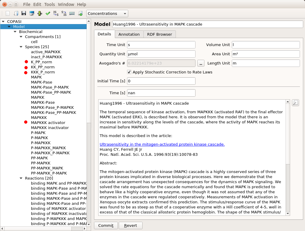
First, we need to have a model to play with. The post will use the model of MAPK signalling published by Huang and Ferrell in 1996. You can find it in BioModels where can download the SBML version and import it in COPASI. Throughout this post, I will assume the reader masters the basic usage of COPASI (create reactions, run simple simulations, etc.). You will find some introductory videos about this user-friendly, versatile, and powerful tool on their website.
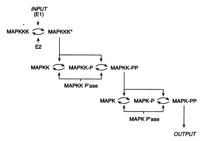
The model presents the three-level cascade activating MAP kinase. MAPK, MAPKK, and MAPKKK mean Mitogen-activated protein kinase, Mitogen-activated protein kinase kinase, and Mitogen-activated protein kinase kinase kinase, respectively. Each curved arrow below represents three elementary reactions: binding and unbinding of the protein to an enzyme, and catalysis (addition or removal of a phosphate).
The top input E1 (above) is called MAPKKK activator in the model. To visualise the results, we will follow the normalised values for the active (phosphorylated) forms of the enzymes K_PP_norm, KK_PP_norm and K_P_norm, that are just the sums of all the molecular species containing the active forms divided by the sums of all the molecular species containing the enzymes (NB: Throughout the screenshots, the red dots are added by myself and not part of COPASI’s GUI).
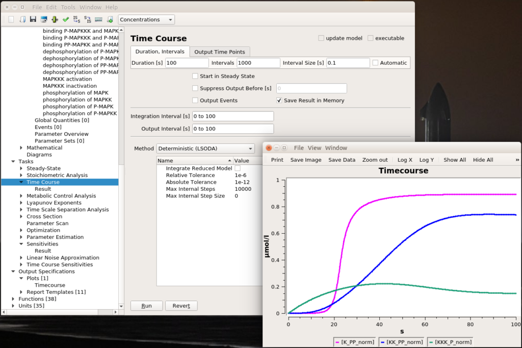
Let’s run a numerical simulation of the model. Below you see the activation of the three enzymes, with the swift and supra-linear activation of the bottom one, MAPK, one of the hallmarks of the cascade (the others being an amplification of the signal and an ultrasensitive dose-response which allows to fully activate MAPK with only a touch of MAPKKK activation).
Sensitivity analysis
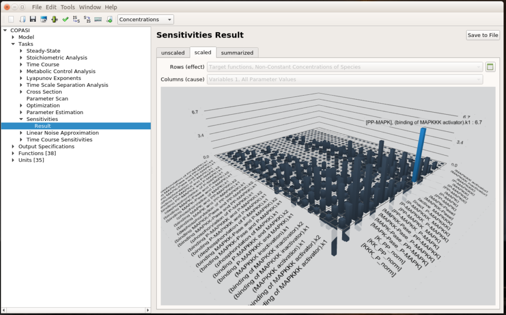
The first question we can ask ourselves is “What are the parameters that values affect the most the output of our system?”. To do so, we can run a sensitivity analysis. COPASI will vary a bit all the parameters and measure the consequences of these changes on the results of a selected task, here the steady-state of the non-constant concentrations of species.
We see that the most important effect is the impact of MAPKKK activator binding constant (k1) on the concentration of PP-MAPK, which happens to be the final output of the signalling cascade. This is quite relevant since the MAPKKK activator binding constant basically transmits the initial signal at the top of the cascade. You can click the small spreadsheet icon on the right to access coloured matrices of numerical results.
Testing values
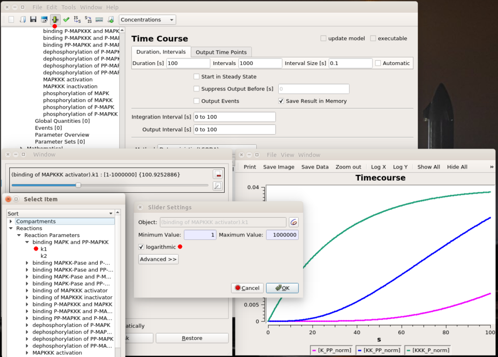
All right, now we know which parameter we want to fiddle with. The first thing we can do is visually look at the effect of modifying the value. We can do that interactively with a “slider“. Once in the timecourse panel, click on the slider icon in the toolbar. You can then create as many sliders as you want to set values manually. Here, I created a slider that can vary logarithmically (advised for most model parameters) between 1 and 1 million. The initial value, used to create the timecourse above, was 1000. We see that sliding to 100 changes the model’s behaviour quite dramatically, with very low enzyme activations. Moving it well above 1000 will show that we increase the speed of activation of the three enzymes, increase the activation of the top enzyme, albeit without significant gain on K-PP, our interesting output.
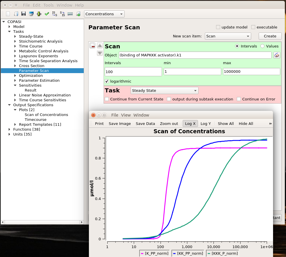
Parameter scans
Playing with sliders is great fun. But this is not very precise. And if we want to evaluate the effect of changing several parameters simultaneously, this can be extremely tedious. However, we can do that automatically thanks to COPASI’s parameter scans. We can actually repeat the simulation with the same value (useful to repeat stochastic simulations), systematically scan parameter values within a range, or sampling them from statistical distributions (and nest all of these). Below, I run a scan over the range defined above and observe the same effect. To visualise the scan’s results, I created a graph that plotted the active enzyme’s steady-state versus the activator binding constant.
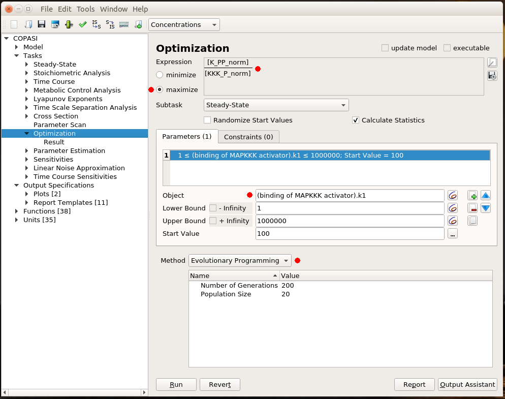
Optimisation
All that is good, but I still have to look at curves or numerical results to find out the best value for my parameter. Ideally, I would like COPASI to hand me directly the value. This is the role of optimisation. Optimisation if made up of two parts: the result I want to optimise and the parameter to change to optimise it. I will not discuss the possibility to optimise a value. There are many cases for which optimisation is just not possible. For instance, it is not possible to optimise the production of phosphorylated MAPK. Whatever upper bound we would fix for the activator binding constant, the optimal value would end up on this boundary. In this example, I decided to maximise the steady-state concentration of K_PP for a given concentration of KKK_P, i.e. getting the most bang for my buck. As before, the parameter I want to explore is the MAPKKK activator binding constant. I fix the same lower and upper bound as before. COPASI offers many algorithms to explore parameter values. Here, I chose Evolutionary Programming, which offers a good balance between accuracy and speed.
The optimal result is 231. Indeed, if we look at the parameter scan plot, we can see that with a binding constant of 231, we get an almost maximal activation of MAPK with minimal activation of MAPKKK. Why is this important? All those enzymes are highly connected and will act on downstream targets right, left, and centre. In order to minimise side effects, I want to activate (or inhibit) protein as little as necessary. Being efficient at low doses also helps with suboptimal bioavailability. And of course, using 100 times less of the stuff to get the same effect is certainly cheaper, particularly for biologics such as antibodies.
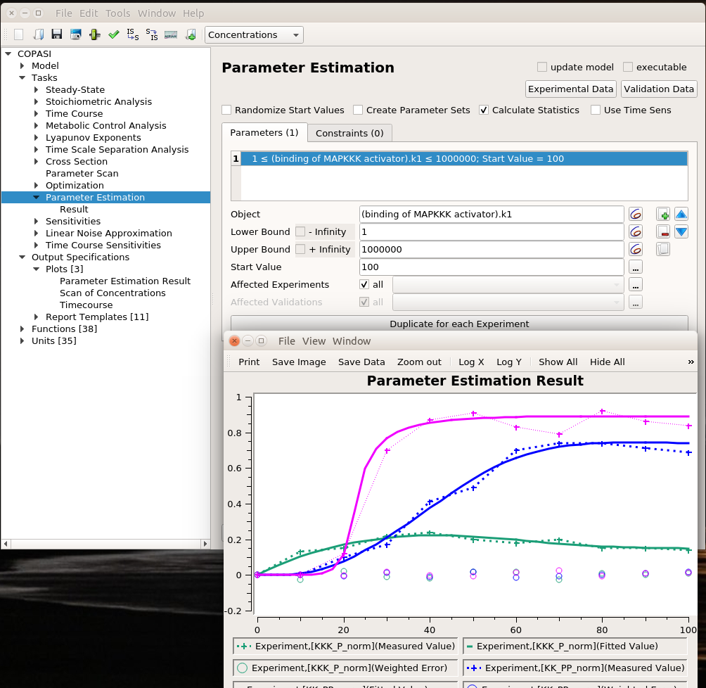
Parameter estimation
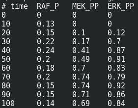
We are now reaching the holy grail of parameter search, which is parameter estimation from observed results. As with optimisation, this is not always possible. It is known as the identifiability problem. Using the initial model, I created a fake noisy set of measurements, which would, for instance, represent the results of Western blot or ELISA using antibodies against phosphorylated and total forms of RAF, MEF, and ERK, which are specific MAPKKK, MAPKK, and MAPK.
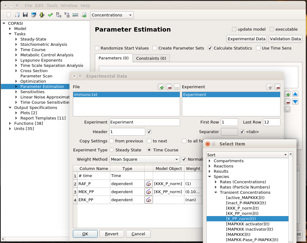
I can load this file (immuno.txt on the screenshot) in COPASI, and map the experimental values (automatically recognised by COPASI) to variables of the model. Note that we can load several files, and each file can contain several experiments.
I can then list the parameters I want to explore, here the usual activator binding constant, between 1 and 1 million. Note that we can use only some of the experiments in the estimation of given parameters. This allows building extremely powerful and flexible parameter estimations.
We can use the same algorithms used in optimisation to explore the parameter space. The plot represents the best solution. Dashed lines link experimental values, continuous lines represent the fitting values, and circles are the error values.
The value estimated by COPASI for the binding constant is 1009. The “experiment” was created with a value of 1000. Not bad.
This concludes our overview of parameter exploration with COPASI. Note that this only brushes up the topic and I hope I picked your curiosity enough for you to read more about it.
Do you have a model that you want to improve? Do you need to model a biological system but do not know the best method or software tool to use? Drop me a message and I will be happy to have a chat.
You are about to embark on a system biology project which will involve some modelling. Here are a few tips to make this adventure more productive and pleasant.
1 – Think ahead
Do not start building the model without knowing where you are going. What do you want to achieve by building this model? Is it only a quick exercise, a one-off? Or do you want this model to become an important part of your current and future projects? Will the model evolve with your questions and the data you acquire? A model with a handful of variables, created to explore an idea quickly, and a model that will be parameterised with experimental measurements, whose predictions will be tested and that will be further expanded are two completely different beasts. Following the 9 tips below in the former case is overkill, a waste of time. However, in the latter case, cutting corners will cause you unending pain when your project unfolds.
2- Focus on the biology
A good systems biology model aims to be anchored in biological knowledge and even (generally) reflects the system’s behaviours’ biological mechanisms. We are using modelling to understand biology and not using biology to illustrate modelling techniques (which is a perfectly respectable activity but not the focus of this blog post). In order to do so, the model must be built from the processes we want to represent (hence complying with the Minimum Information Requested in the Annotation of Models). Therefore, try to build up your model from reactions (or transitions if this is a Petri Net, rules for a Rule-based model, influences for a Logic model), rather than writing directly the equations controlling the evolution of variables.
Another aspect worth a thought is the existence of different “compartments”. In systems biology, compartments are the “spaces” that contain the biological entities represented by your variables (the word has a slightly different meaning in PKPD modelling, meaning the variable itself). Because compartments can have different sizes, these sizes can change, and they can be used to affect other aspects of the models, it is important to represent them correctly, rather than ignoring them altogether, which was the case for decades.
Many tools have been developed to help you build models that way, such as (but absolutely not limited to) CellDesigner and the excellent COPASI. These software tools are, in general, very user-friendly and more approachable for biologists. An extensive list of tools is available from the SBML software guide.
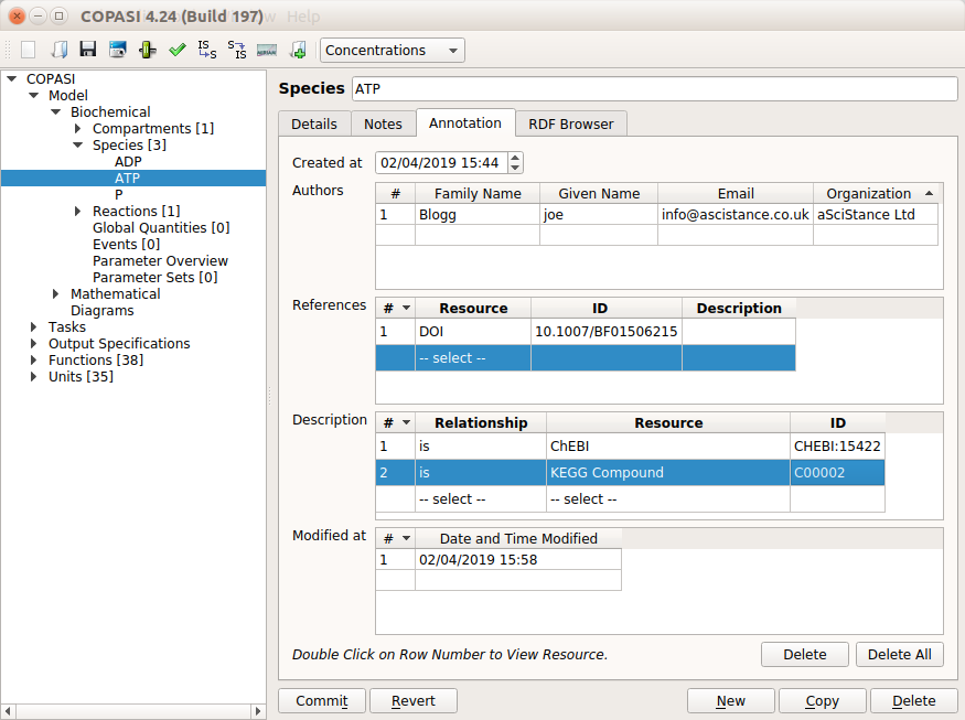
3- Document as you build
Bookkeeping is a cornerstone of any professional activity, and lab notebooks are scientists’ best friends. Modelling is no exception. If you do not log why you created a variable or a reaction, what biological entities they represent, how you chose the initial values or the boundaries for parameter estimation, you will make your life down the line hell. You will not be able to interpret the results of simulations, modify the model, share it with collaborators, write a publication, etc. You must start this documentation as soon as you begin building the model. Memory fades quickly, and motivation even quicker. The biggest self-delusion (or plain lie) is “I am efficient and focused now, and I must get results done. I will clean up and document the model later.” You will most probably never clean up and document the model. And if you do, you will suffer greatly, trying to remember why the heck you made those choices before.
Several software tools, such as COPASI, provide means of annotating every single element of a model, either with free text, or with controlled annotations. Alternatively, you can use regular electronic notebooks, Google docs, and spreadsheets if you work with others etc. Anything goes, as far as you do create this documentation. Note that you can later share model and documentation at once, either with the documentation included in the model (for instance, in SBML notes and annotation elements) or with model and documentation shared as a single COMBINE Archive.
4- Choose a consistent naming scheme
This sounds like a mundane concern. But it is not! Variable and parameter names are the first layer of documentation (see tip 3). It also anchors your model in biology (tip 2). A naming scheme that is logical and consistent while easy to remember and use will also greatly facilitate future extensions of your model (tip 1). NB: we do not want to open a debate “identifiers versus accession number versus usable name” or the pros and cons of semantics in identifiers (see the paper by McMurry et al for a great discussion on that topic). Here, we talk about the short names one sees in equations, model graphs, etc.
Avoid very long names if not needed (“adenosine triphosphate”), but do not be over-parsimonious (“a”). “ATP” is fine. Short, explicit, clear for most people within a given context. Reuse common practices if possible, even if they are not official. For instance, uppercase K is mostly used for equilibrium constants, lowercase k for rate constants. A model using “Km” for the rate constant of DNA methylase and “kd” for its dissociation constant from DNA would be pretty confusing. Be consistent in the naming. If non-covalent complexes are denoted with an underscore, A_B being a complex between A and B, and hyphens denote covalent modifications, A-P representing the phosphorylated form of A, do not use CDP for the phosphorylated form of the complex between C and D (or, heaven forbid, C-D_P !!!)
5- Choose granularity and independent variables wisely
We often make two mistakes when describing systems in biology mathematically. The first one is a variant of the “spherical cow“. In order to facilitate the manipulation of the model, it is very tempting to create as few independent variables as possible (by variable, we mean here the things we can measure and predict). Those variables can be combinations of others, combinations sometimes only valid in specific conditions. Such simplifications make exploring the different behaviours easier, for instance, with phase portraits and bifurcation plots. A famous example is the two variable version of the cell cycle model by John Tyson in 1991. However, the hidden constraints might not allow the model to reproduce all the behaviours displayed by the biological system. Moreover, reverse engineering the variables to interpret the results could be difficult.
The second, mirroring, mistake is to try modelling the biological system in exquisite details, representing all our knowledge and thus creating too many variables. Even if the mechanisms underlying the interactions between those variables were known (which is most often not the case), the resulting model often contains too many degrees of freedom, effectively allowing any behaviour to be reproduced with some parameter values (making it impossible to falsify). It also becomes challenging to accurately determine the values of all parameters based on a limited number of independent measurements.
It is therefore paramount to choose the right level of granularity. There is no universal and straightforward solution, and we can encounter extreme cases. d’Alcantara et al 2003 represented calmodulin is represented by two variables (total concentration and concentration of active molecules). In Stefan et al 2008, calmodulin is represented by 96 variables (all calcium-binding combinations plus binding to other proteins and different structural conformations). Nevertheless, both papers study the biological phenomenon.
The right answer is to pick the variable granularity depending on the questions asked and the data available. A rule of thumb is to start with a small number of variables that can be matched (directly or via mathematical transformations) with the quantities you have measurements for. Then you can progressively make your model more complex and expressive as you move on while keeping it identifiable.
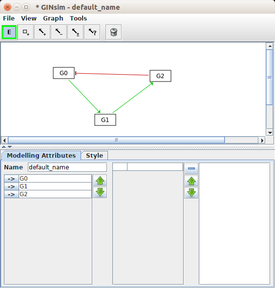
6- Create your relationships
Once you have defined your variables, you can create the necessary relationships, which are all the mathematical constructs that link variables and parameters together. Graphical software such as CellDesigner or GINsim permit to draw the diagrams representing the processes or the influences respectively.
Note that some software tools provide shorthand notations that permit the creation of variables and parameters directly when writing the reactions. This is very handy for creating small models instantly. However, I would refrain from doing so if you want to document your model properly (it also makes it easier to create spurious variables and “dangling ends” through typos in the variable names).
Working on the relationships after defining the variables also easily permits the model’s modification. For example, you can add or remove a reaction without having to go through the entire model as you would with a list of ordinary differential equations.
7- Choose your math
The beauty of mathematical models is that you can explore a large diversity of possible linkages between molecular species, actual mechanisms hidden behind the “arrow” representing a process. A transformation of X in a compartment into Y in another compartment can be controlled for instance by a constant flux (don’t do that!), a passive diffusion, a rate-limited transport, or even exotic higher-order kinetics. At that point, we could write: [insert clone of tip 5 here]. Indeed, while the mathematical expressions you choose can be arbitrarily complex, the more parameters you have, the harder it will be to find proper values for them.
If the model is carefully designed, switching between kinetics should not be too difficult. A useful habit to take is to preferentially use global parameters (which scope is the entire model/module) rather than parameters defined for a given reaction/mathematical expression. Doing so will, of course, ease the use of the parameter in different expressions and facilitate the documentation and ease future model extensions, for instance, where a parameter no longer has a fixed value but is affected by other things happening in the model.
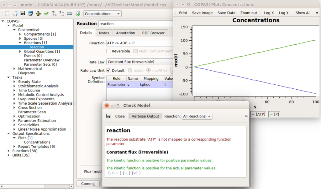
8- Plug holes and check for mistakes
Now that you have your shiny model, you need to make sure you did not forget to close a porthole that would sink it. Do you have rate laws generating negative concentrations? Conversely, does your model generate umpteen amounts of certain molecules which are not consumed, resulting in preposterous concentrations? Software like COPASI have checks for this kind of thing. In the example below, I created a reaction that consumes ATP to produce ADP and P, with a constant flux. This would result in infinite concentrations of ADP and infinitely negative concentrations of ATP. COPASI catches it, albeit returning a message that could be clearer.
Ideally, a model should be “homeostatic”. All molecular species should be produced and consumed. Pure “inputs” should be produced by creation/import reactions, while pure “outputs” should be consumed by degradation/export reactions. Simulating the model would not lead to any timecourse tending to either +∞ or -∞.
9- Create output
“A picture is worth a thousand words”, and the impact of the results you obtained with such a nice will be greater if served in clear, attractive and expressive figures. Timecourses are useful. But they are not always the best way to present the key message. You want to show the effect of parameter values on molecular species’ steady-states? Try parameter scanning plots, and their derivatives, such as bifurcation plots. Try phase-portraits. Distributions of concentrations during stochastic simulations or after ensemble simulations can be represented with histograms. And why being limited to 2D-plots? Use 3D plots and surfaces instead, possibly in conjunction with interactive display (plot.ly …).
10- Save your work!
Finally, and this is quite important, save often and save all versions. Models are code, and code must be versioned. You never know when you will realise you made a mistake and will want to go back a few steps and start exploring a different direction. You certainly do not want to start all over again. Recent work explored ways of comparing model versions (see the works from the Waltemath group, for instance). But we are still some way off the possibility of accurately “diff and merge” as it is done on text and programming code. The safest way is to save all the significant versions of a model separately.