By Nicolas Gambardella
In the absence of information regarding the structure of variability (whether intrinsic noise, technical error or biological variation), one very often assumes, consciously or not, a normal distribution, i.e. a “bell curve”. This is probably due to an intuitive application of the central limit theorem which stipulates that when independent random variables are added, their normalized sum tends toward such a normal distribution, even if the original variables themselves are not normally distributed. The reasoning then goes that any biological process is the sum of many sub-processes, each with its own variability structure, therefore its “noise” should be Gaussian.
Although that sounds almost common sense, alarm bells start ringing when we use such distributions with molecular measurements. Firstly, a normal distribution ranges from -∞ to +∞. And there is no such things as negative amounts. So, at most, the variability would follow a truncated normal distribution, starting at 0. Secondly, the normal distribution is symmetrical. However, in everyday conversation, the biologists will talk of a variability “reaching twofold”. For a molecular measurement, a two-fold increase and a two-fold decrease do not represent the same amount. So there is an asymmetric notion here. We are talking about linking the addition and removal of the same “quantum of variability” to a multiplication or division by a same number. Immediately logarithms come to mind. And log2 fold changes are indeed one of the most used method to quantify differences. Populations of molecular measurements can also be – sometimes reasonably – fitted with log-normal distributions. Of course, several other distributions have been used to fit better cellular contents of RNA and protein, including the gamma, Poisson and negative binomial distributions, as well as more complicated mix.
Let’s look at some single-cell gene expression measurements. Below, I plotted the distribution of read counts (read counts per million reads to be accurate) for four genes in 232 cells. The asymmetry is obvious, even for NDUFAB1 (the acyl carrier protein, central to lipid metabolism). This dataset was generated using a SmartSeq approach and Illumina HiSeq sequencing. It is therefore likely that many of the observed 0 are “dropouts”, possibly due to the reverse transcriptase stochastically missing the mRNAs. This problem is probably even amplified with methods such as Chromium, that are known to detect less genes per cell. Nevertheless, even if we remove all 0, we observe extremely similar distributions.
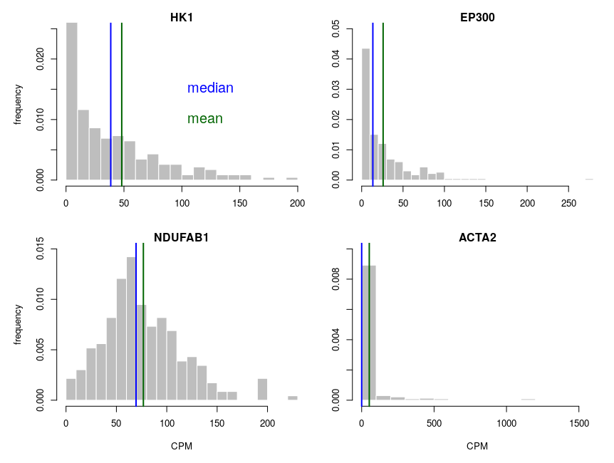
One of the important consequences of the normal distribution’s symmetry, is that mean and median of the distribution are identical. In a population, we should have the same amounts of samples presenting less and presenting more substance than the mean. In other words, a “typical” sample, representative of the population, should display the mean amount of the substance measured. It is easy to see that this is not the case at all for our single cell gene expressions. The numbers of cells expressing more than the mean of the population are 99 for ACP (not hugely far from the 116 of the median), 86 for hexokinase, 78 for histone acetyl transferase P300 and 30 for actin 2. In fact, in the latter case, the median is 0, mRNAs having been detected in only 50 of the 232 cells ! So, if we take a cell randomly in the population, most of the time it presents a count of 0 CPM of actin 2. The mean expression of 52.5 CPM is certainly not representative!
If we want to model the cell type, and provide initial concentrations for some messenger RNAs, we must use the median of the measurements, not the mean (of course, the best route of action would be to build an ensemble model, cf below). The situation would be different if we wanted to model the tissue, that is a sum of non individualised cells representative of the population.
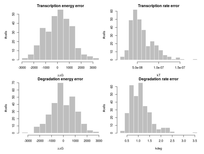
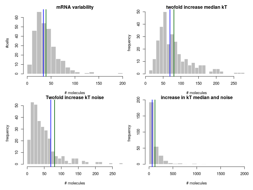
To explain how such asymmetric distributions can arise from noise following normal distributions, we can build a small model of gene expression. mRNA is transcribed at a constant flux, with a rate constant kT. It is then degraded following a unimolecular decay with rate kdeg (chosen to be 1 on average, for convenience). Both rate constants are computed from energies, following the Arrhenius equation, k = Ae-(E/RT), where R is the gas constant, 8.314 and T is the temperature, that we set at 310 K (37 deg C). To simplify we’ll just set the scaling factor A to 1, assuming it is included in the reference energy. E is 0 for degradation, and we modulate the reference transcription energy to control the level of transcript. Both transcription and degradation energy will be affected by normally distributed noises that represent differences between cells (e.g. concentration and state of enzymes). So Ei = E + noise. Because of Arrhenius equation, the normal distributions of energy are transformed into lognormal distributions of rates. Below I plot the distributions of the noises in the cells and the resulting rates.
The equilibrium concentration of the mRNA is then
In summary:
- Means of single cell molecular measurements are not a good way of getting a value representing the population;
- Comparing the means of single measurements in two populations does not provide an accurate estimation of the underlying changes;