By Nicolas Gambardella
COVID-19 pandemics put mathematical models of biological relevance all over daily newspapers and TV news, raising their profile for the non-scientists. In the life sciences, while mathematical models have always been at the core of some disciplines, such as genetics, they really became mainstream with the rebirth of systems biology a couple of decades ago. However, there are many different modelling approaches, and even specialists often ignore methods they do not use regularly or have not been taught.
After a historical overview, this blog post will then attempt to classify the main types of models used in systems biology according to their principal modalities.
What is the goal of using mathematical models in the life sciences in the first place? Three main aims came out roughly sequentially during the XX century, following the path physics followed over the past two millennia. First, mathematics helps describe the structure and dynamics of living forms and their productions. These models may rely on supposed underlying laws, be purely descriptives, such as the allometric laws. A great example is the famous book “On Growth and Form” by D’Arcy Thompson, attempting to understand living forms based on physical laws.
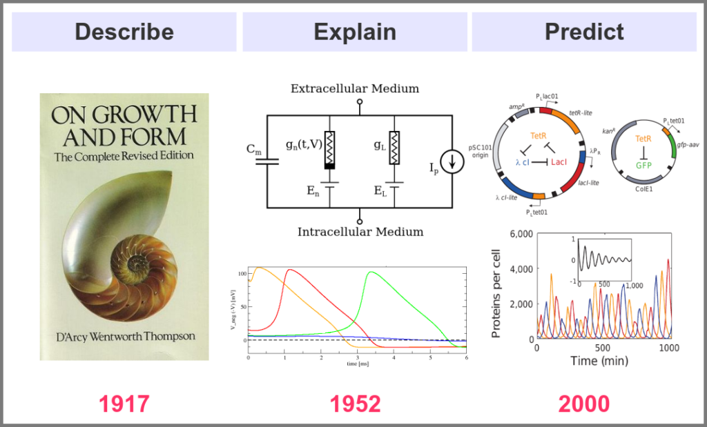
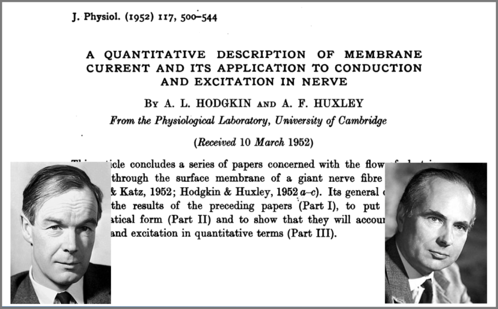
The second aim is to explain the shape and function of living forms. How do the properties of life’s building blocks explain what we can observe? In their masterwork, Alan Hodgkin and Andrew Huxley predicted the existence of ionic channels within the cell membrane and, using a mathematical model, explained how neurons generate action potentials (a work for which they got the Nobel prize).
Finally, can we predict how a system will behave, and can we invent new systems that will behave the way we want them to? This is the purpose of synthetic biology, exemplified in the figure below by the pioneering work of Michael Elowitz and Stanislas Leibler, who built the “repressilator”, a synthetic construct exhibiting sustained oscillations maintained through generations of bacteria.
Obviously, there are no strict boundaries between the three aims, and most models seek to describe, explain, and predict the structures and behaviours of living systems.
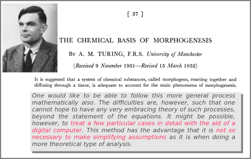
A major shift in the use of mathematical models was the introduction of numerical simulations, made feasible by the invention of computers. The benefits have been laid out by one of the inventors of such computers in an article that indeed contained complex mathematical models but no simulations. In his famous 1952 paper introducing morphogens, Alan Turing suggested that using a digital computer to simulate specific cases of a biological system would allow avoiding the oversimplifications required by analytic solutions.
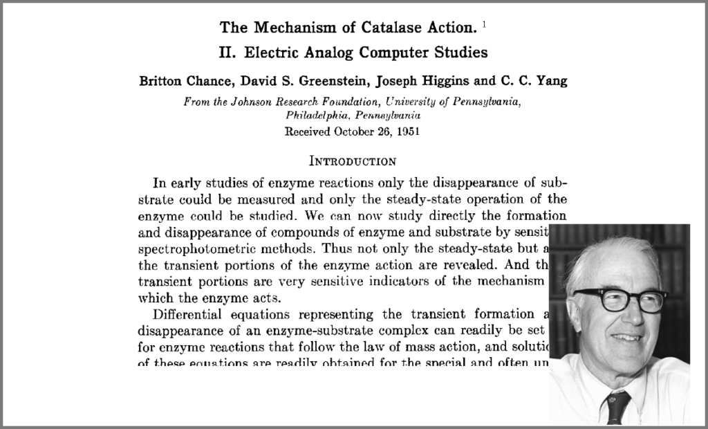
This wish was granted the very same year first by Britton Chance, who built a computer (an analogue one at the time) specifically to solve a differential equation model of a small biochemical pathway.
1952 was also when Hodgkin and Huxley published the action potential model mentioned above, a real Annus Mirabilis for computational modelling in the life sciences.
Before going further, we should ask ourselves, “what is a mathematical model”? According to Wikipedia (as of 4th July 2022), A mathematical model is a description of a system using mathematical concepts and language. I consider that three essential categories of components form mathematical models in systems biology.
Variables represent what we want to know or what we want to compare with the observations. They can characterise a physical entity, e.g., the concentration of a substance, the length of an object or the duration of an event, or be derived from the model itself, for instance, the maximum velocity of an enzymatic reaction.
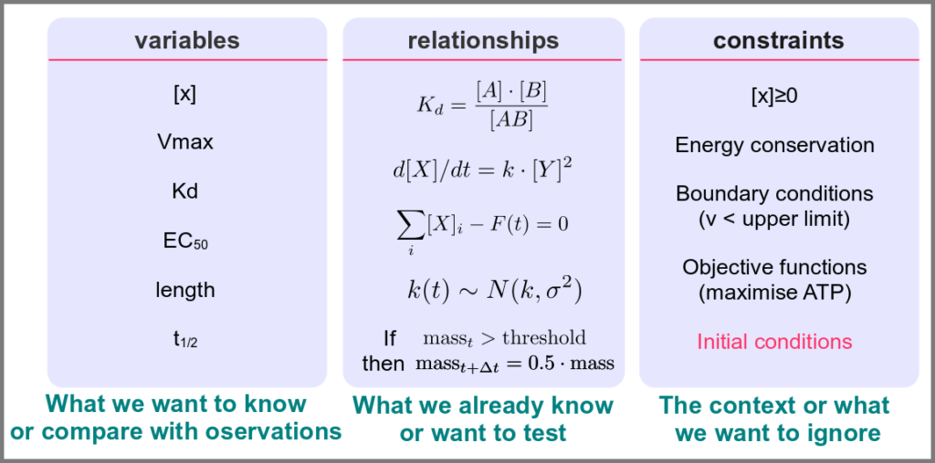
Relationships mathematically link variables together and represent what we know or what we want to test. They can be static, an affinity constant linked to concentrations or dynamic, such as a rate of change depending on concentrations. Relationships are not necessarily equations. For instance, a sampling might link a variable to a statistical distribution, and logic models use logical statements to attribute values to variables.
Finally, a much-underestimated category is formed by constraints put on the model. Those represent the context of the modelling project or what we consciously decide to ignore. Some constraints are properties of the world, e.g., a concentration must always be positive, the total energy is conserved, and some are properties of the model, such as boundary conditions and objective functions for optimisation procedures. Initial conditions – the values of variables before starting a numerical simulation – are also crucial since a given model might behave differently with different initial conditions, even if neither variables nor relationships are changed.
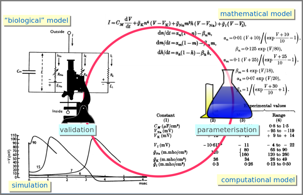
However, the mathematical model itself is only one brick of a systems biology’s modelling and simulation project as in any natural science domain. Since these models aim to be mechanistic, i.e., anchored in underlying molecular, cellular, tissular, and physiological processes, the first step is to conceptualise a “biological model”. For instance, a biochemical pathway will be a collection of chemical reactions. In the case of Hodgkin and Huxley, who did not know the underlying molecules, the mechanism was based on an electrical analogy, ionic channels being represented by electrical conductances. The “mathematical model” is made up of mathematical relationships linking the variables and constraints. A “computational model”, using the “mathematical model” in conjunction with observed or estimated values, is then simulated. The result is compared with observations, and the loop is iterated.
Now let’s explore the different facets of models used in systems biology, and marvel at their diversity
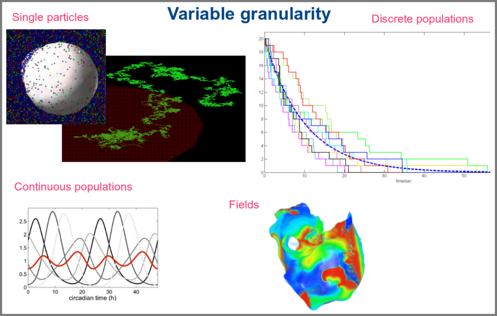
The variables of a model can represent biological reality at different granularities. In some logical models (often wrongly called Boolean networks), a variable can represent a state, such as presence or absence, 1, 2, 3. Detailed models at the “mesoscopic scale” might represent individual molecules, where a separate variable represents every single particle. Variables can also represent discrete populations of molecules, for instance, the number of molecules of a given chemical class, whose evolution is simulated by stochastic algorithms. In chemical kinetics, the variables whose change is determined using ordinary differential equations often represent continuous concentrations. Finally, some models gloss over the physical parts altogether and use fields to represent what could happen to them.
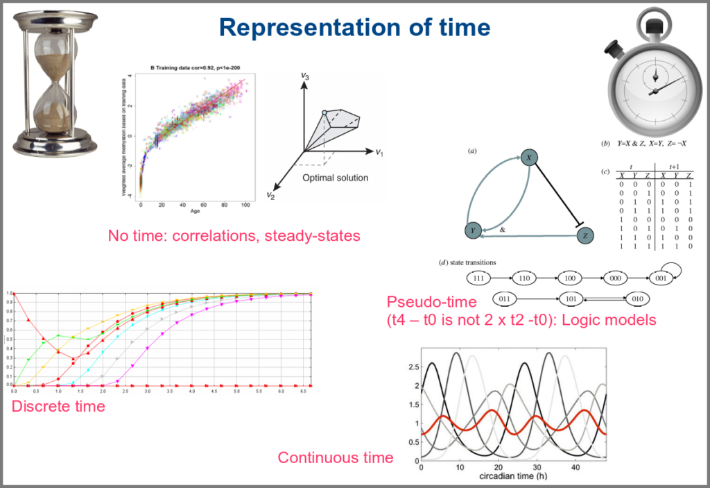
Numerical simulations most often represent the evolution of variable values over “time”. However, the granularity of this “time” may vary. At an extreme, we have models with no representation of time, such as regression models, or implicit representation of time, such as steady-states models. In logical models, as in Petri Net, simulations usually progress along a pseudo-time, where one cannot compare numbers of steps. Time can be discrete, numerical simulations computing a system’s state at fixed intervals, for instance, one second. Finally, models can consider time as continuous, simulations being iterated at various timepoints decided by numerical solvers (note that software might still return results at fixed intervals).
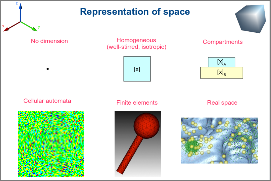
Spacetime being a thing, we also have as many different representations of space. Starting with no space at all, for instance, in noncompartmental analyses of pharmacokinetic models. Space can also be represented by a single homogenous (well-stirred) and isotropic compartment or several of them connected by variables and relationships (multi-compartment models, a.k.a. bathtub models). Cellular automata constitute a particular case, where each compartment is also a model variable whose status depends on its neighbours’. An extension of the multi-compartment modelling represents realistic biological structures using finite elements, each considered homogeneous and isotropic. Finally, space might be represented by continuous variables, where the trajectory of each molecule can be simulated.
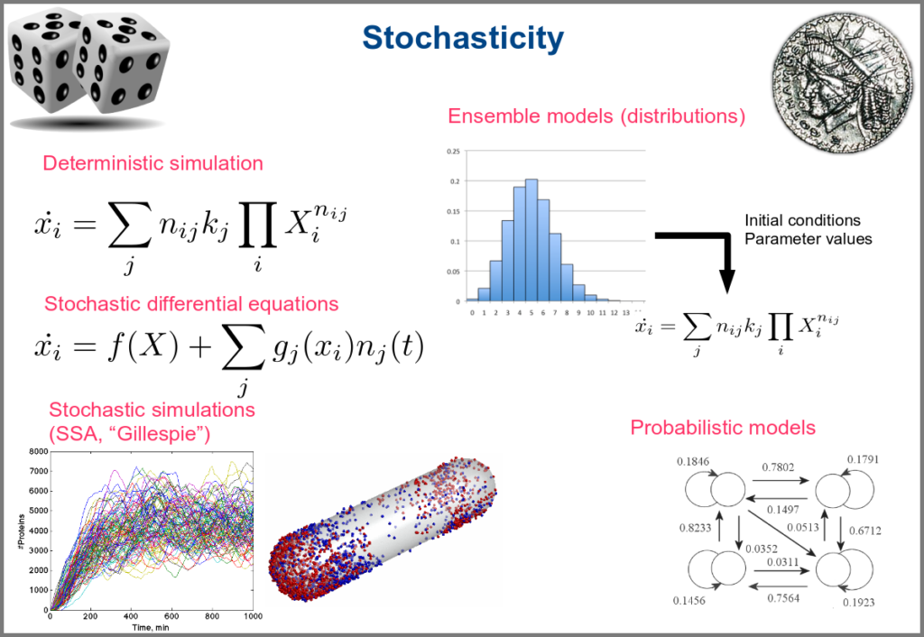
Variability and noise are unavoidable parts of any observation of the natural world, including living systems. Variability can be extrinsic (e.g., due to technical variability), or intrinsic (e.g., actual differences between cells or samples). True noise depends on the size of the system. Taking all those into account in the models can thus be important, and different approaches present different levels and types of stochasticity. As with the other modalities above, stochasticity might be entirely absent, models and simulations being deterministic. One can add different and arbitrary types of noise to simulations with stochastic differential equations. The stochastic aspect might instead emerge directly from the structure of the model, as with the Stochastic Simulation Algorithms (a.k.a. algorithms of the “Gillespie” type). Variability can also be taken into account prior to the simulations, for instance, by sampling initial conditions from distributions, as with ensemble modelling. Finally, in probabilistic models such as Markov models, the entire iteration of the system is based on the probabilities of switching states.
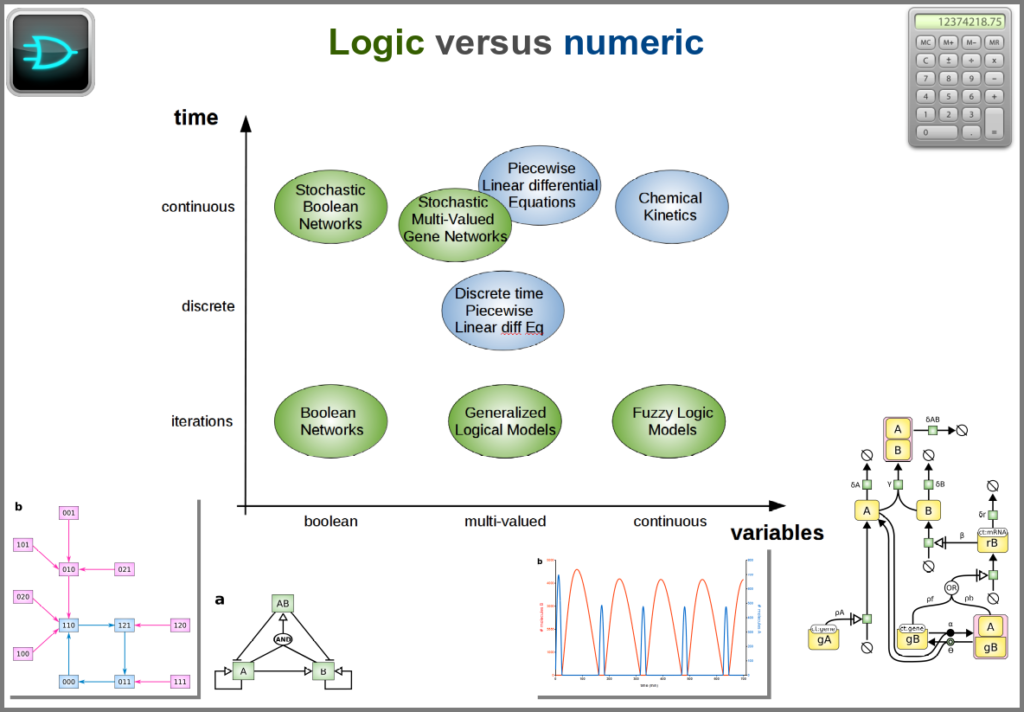
Finally, there are two large families of models based on the type of algorithms used to update the variables. One can compute a variable’s new value by calculating its value either using numerical combinations of previous variables’ values or logic rules taking into account other variable states. Contrary to widespread belief, not all logic models use pseudo-time and Boolean variables. Stochastic Boolean networks can use continuous time, and fuzzy logic models can base their decision on continuous variable values.
Those modalities can be combined in many ways to produce an extremely rich toolkit of modelling approaches. One of the most frequent sources of pain when modelling biological systems is to start with a methodological a priori, often because we are comfortable with an approach, we have the necessary software, or we don’t know better. Doing so can result in under-determined models, endless iterations and failure to get any result. The choice of a modelling approach should be first and foremost based on:
1) the question asked, and
2) the data available to build and validate the model.
References
Chance, B., Greenstein, D. S., Higgins, J. & Yang, C. C. (1952) The mechanism of catalase action. II. Electric analog computer studies. Arch. Biochem. Biophys. 37: 322–339. doi:10.1016/0003-9861(52)90195-1
Hodgkin, A.L., Huxley, A.F. (1952). A quantitative description of membrane current and its application to conduction and excitation in nerve. The Journal of Physiology. 117 (4): 500–44. doi:10.1113/jphysiol.1952.sp004764
Stanislas Leibler; Elowitz, Michael B. (2000-01-20). “A synthetic oscillatory network of transcriptional regulators”. Nature 403 (6767): 335–338. doi:10.1038/35002125.
Thompson, D. W., 1917. On Growth and Form. Cambridge University Press.
Turing, A. M. (1952). “The chemical basis of morphogenesis”. Philosophical Transactions of the Royal Society of London B. 237 (641): 37–72. doi:10.1098/rstb.1952.0012.