When I receive manuscripts to edit, I am often surprised to see how poor the figures are, particularly the plots. They are confusing, lack colours (and when in colour are not colour-blind-friendly), the font size is too small, etc. Your figures convey much more than the results. For better or worse, they will bias the reader’s mind about your results’ quality and affect their confidence in your conclusions.
It is not hard to improve our plots, though. We must think about the readers and what we like in other people’s plots. Let’s take the example of a histogram. I’ll use the single cell RNAseq data already presented in my post about medians and means. We want to see if the distribution of gene expressions across many single cells corresponds to a lognormal law. We will plot the expression of four genes, their calculated mean and median, a fitted lognormal distribution and the mean and median of the latter. (NB: We know gene expression does not really follow a lognormal distribution, and comparing distributions is not the proper way to determine if a dataset corresponds to a distribution. If you are interested, have a look at Q-Q plots and the Shapiro-Wilk test.)
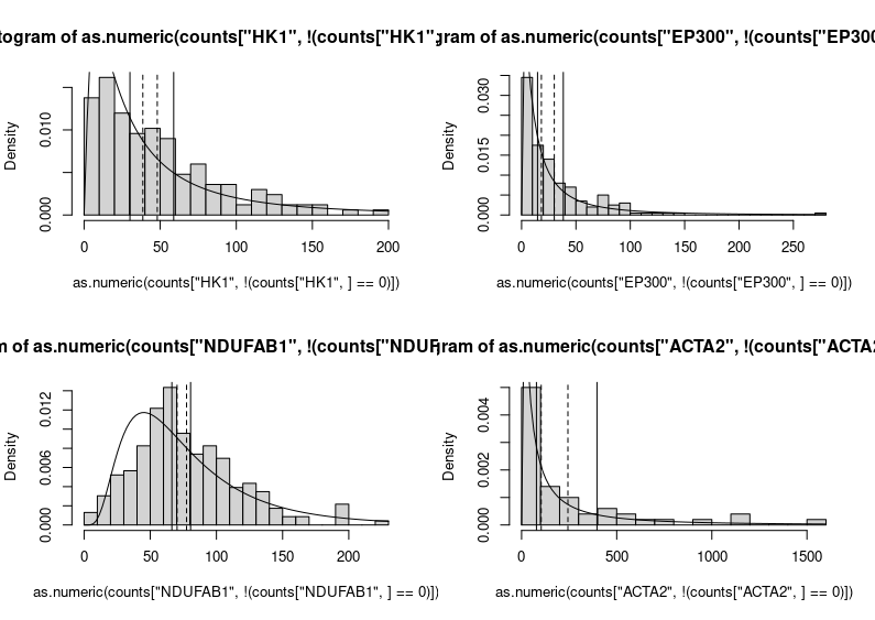
Here we go.
Yikes!
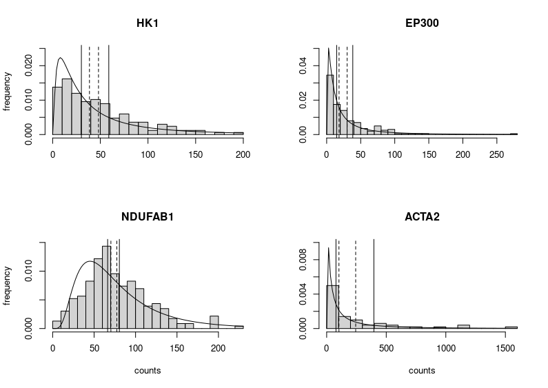
This is horrendous. The fitted distributions are cut, legends are unreadable, and all that grey, so depressing. Let’s improve the figure by choosing different limits for the Y axes to make the entire fitted distributions visible. We can also improve each plot’s title and the labels of the axes. We do not need the latter on each subplot (we can also change the label “density” produced by plotting the fitted distribution into “frequency”, the label we would get by plotting only the histograms. Indeed, the height of the boxes represents the fraction of cells presenting the expression plotted on the X axis.
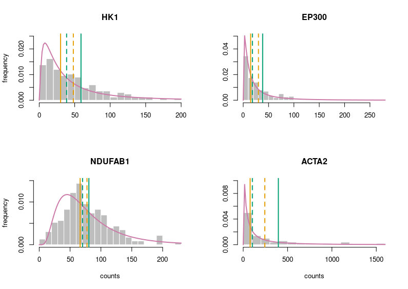
Better. But still very grey. Let’s put some colours on this plot. Those colours are colour-blind-friendly (thanks to the “Colour universal design” of Masataka Okabe and Kei, Ito).
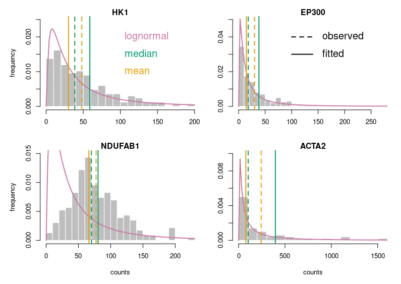
Now, this looks publication-grade. I feel there is still too much white space, so let’s tighten that a bit and add legends.
Of course, for this blog post, I voluntarily started with base R. Using ggplot2 in the first place would have provided a much better starting point. I just wanted to make a point. Here is the code:
# counts is a dataframe with genes in rows and cells in columns

# fitting the counts of hexokinase across all cells to a lognormal law; only consider non-zero values
# (the other four genes are fitted using the same code)
fit_params_HK1 <- fitdistr(as.numeric(counts["HK1",!(counts["HK1",]==0)]),"lognormal")

# to get a 2 by 2 figure without too much empty white space
par(mfrow=c(2,2),
    oma = c(1,1,1,1) + 0.0,
    mar = c(4,4,1,0) + 0.0)

# plot for the hexokinase (the other four genes are plotted using the same code)
# histogram of cell counts
hist(as.numeric(counts["HK1",!(counts["HK1",]==0)]),breaks=20,prob=TRUE,
     col="gray", border = "white",
     main="HK1",xlab=NULL,ylab="frequency",ylim=c(0,0.025))
# lognormal distribution fitted on the counts
curve(dlnorm(x, fit_params_HK1$estimate[1], fit_params_HK1$estimate[2]), col=rgb(204/255,121/255,167/255), lwd=2, add=T)

# observed median and mean
abline(v=median(as.numeric(counts["HK1",!(counts["HK1",]==0)])), col=rgb(0/255,158/255,115/255),lwd=2,lty=2)
abline(v=mean(as.numeric(counts["HK1",!(counts["HK1",]==0)])), col=rgb(230/255,159/255,0/255),lwd=2,lty=2)

# median and mean of the fitted law. remember that the median of a lognormal distributed variable is the mean
# of the log of the variable (meanlog), and its mean is meanlog+sdlog^2/2
abline(v=exp(fit_params_HK1$estimate[1]+(fit_params_HK1$estimate[2])^2/2), col=rgb(0/255,158/255,115/255),lwd=2)
abline(v=exp(fit_params_HK1$estimate[1]), col=rgb(230/255,159/255,0/255),lwd=2)

# plotting the legends for the colours
text(100, 0.02, labels = "lognormal", pos = 4, cex = 1.5, col=rgb(204/255,121/255,167/255))
text(100, 0.015, labels = "median", pos = 4, cex = 1.5, col=rgb(0/255,158/255,115/255))
text(100, 0.01, labels = "mean", pos = 4, cex = 1.5, col=rgb(230/255,159/255,0/255))

# plotting the legend located on the histone acetylase EP300
segments(100,0.04, 140,0.04,col = "black", lty = 2,lwd=2)
segments(100,0.03, 140, 0.03,col = "black", lty = 1,lwd=2)
text(150, 0.04, labels = "observed", pos = 4, cex = 1.5, col="black")
text(150, 0.03, labels = "fitted", pos = 4, cex = 1.5, col="black")
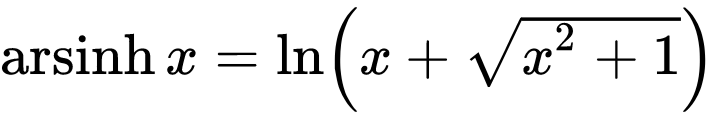
Do you need to normalize data quickly but are bothered by null or negative values? You can use the Inverse hyperbolic sine, Arsinh, function instead of a simple log function. This approach also allows for treating differently small and high values. Arsinh is defined as:
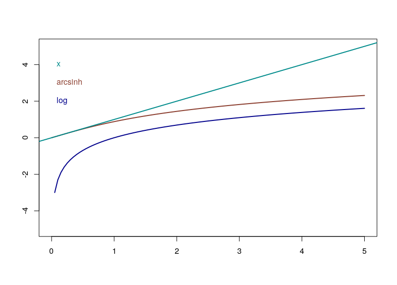
Firstly, since x+sqrt(x²+1) is always strictly positive, arsinh is defined for all real values, contrary to log, which is only defined for strictly positive numbers. Furthermore, as can easily be seen, for small values of x, the function tends to ln(x+1), something often used to overcome the 0 measurements. For large values of x, arsinh(x) progresses as log(x).
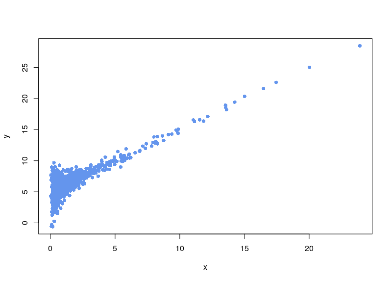
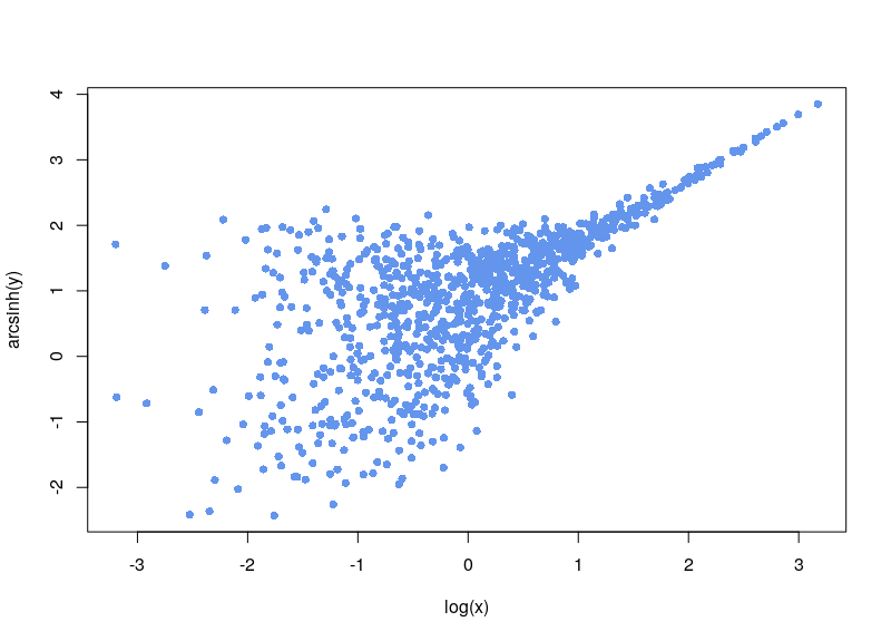
Let’s say we have a dataset that is quite noisy, with unevenly spread sampling, and that includes an unwanted baseline. Here is a made-up dataset:
To create it, we generated 1000 lognormal-distributed sampling values x. The variable value is equal to the sampling value, plus a random noise in which the standard deviation varies as the ratio of sqrt(x)/x (biological noise), plus a noisy constant technical baseline (5 plus a normal noise with SD=0.01).
We are clever, and notice the background noise, so we subtract it:
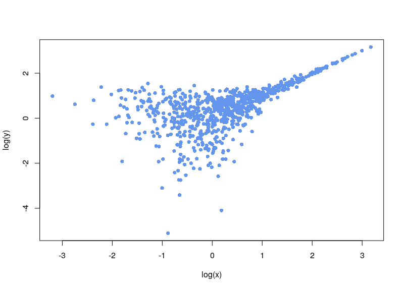
Now, the first issue is that plenty of values are negative. In some cases, your normalization will fail. Sometimes, the normalization will proceed, ditching values (as R says, “Warning message: NaNs produced”). As can be seen below, there is a large area sparsely populated on the left for low values of x.
If, on the contrary, we use arsinh, we rescue all those values.
In the absence of information regarding the structure of variability (whether intrinsic noise, technical error or biological variation), one very often assumes, consciously or not, a normal distribution, i.e. a “bell curve”. This is probably due to an intuitive application of the central limit theorem which stipulates that when independent random variables are added, their normalized sum tends toward such a normal distribution, even if the original variables themselves are not normally distributed. The reasoning then goes that any biological process is the sum of many sub-processes, each with its own variability structure, therefore its “noise” should be Gaussian.
Although that sounds almost common sense, alarm bells start ringing when we use such distributions with molecular measurements. Firstly, a normal distribution ranges from -∞ to +∞. And there is no such things as negative amounts. So, at most, the variability would follow a truncated normal distribution, starting at 0. Secondly, the normal distribution is symmetrical. However, in everyday conversation, the biologists will talk of a variability “reaching twofold”. For a molecular measurement, a two-fold increase and a two-fold decrease do not represent the same amount. So there is an asymmetric notion here. We are talking about linking the addition and removal of the same “quantum of variability” to a multiplication or division by a same number. Immediately logarithms come to mind. And log2 fold changes are indeed one of the most used method to quantify differences. Populations of molecular measurements can also be – sometimes reasonably – fitted with log-normal distributions. Of course, several other distributions have been used to fit better cellular contents of RNA and protein, including the gamma, Poisson and negative binomial distributions, as well as more complicated mix.
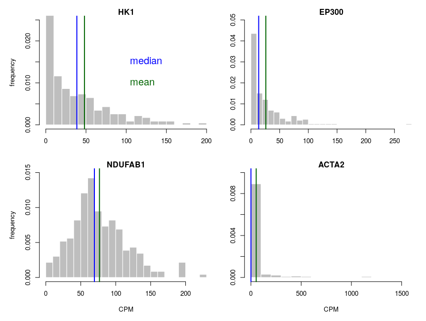
Let’s look at some single-cell gene expression measurements. Below, I plotted the distribution of read counts (read counts per million reads to be accurate) for four genes in 232 cells. The asymmetry is obvious, even for NDUFAB1 (the acyl carrier protein, central to lipid metabolism). This dataset was generated using a SmartSeq approach and Illumina HiSeq sequencing. It is therefore likely that many of the observed 0 are “dropouts”, possibly due to the reverse transcriptase stochastically missing the mRNAs. This problem is probably even amplified with methods such as Chromium, that are known to detect less genes per cell. Nevertheless, even if we remove all 0, we observe extremely similar distributions.
One of the important consequences of the normal distribution’s symmetry, is that mean and median of the distribution are identical. In a population, we should have the same amounts of samples presenting less and presenting more substance than the mean. In other words, a “typical” sample, representative of the population, should display the mean amount of the substance measured. It is easy to see that this is not the case at all for our single cell gene expressions. The numbers of cells expressing more than the mean of the population are 99 for ACP (not hugely far from the 116 of the median), 86 for hexokinase, 78 for histone acetyl transferase P300 and 30 for actin 2. In fact, in the latter case, the median is 0, mRNAs having been detected in only 50 of the 232 cells ! So, if we take a cell randomly in the population, most of the time it presents a count of 0 CPM of actin 2. The mean expression of 52.5 CPM is certainly not representative!
If we want to model the cell type, and provide initial concentrations for some messenger RNAs, we must use the median of the measurements, not the mean (of course, the best route of action would be to build an ensemble model, cf below). The situation would be different if we wanted to model the tissue, that is a sum of non individualised cells representative of the population.
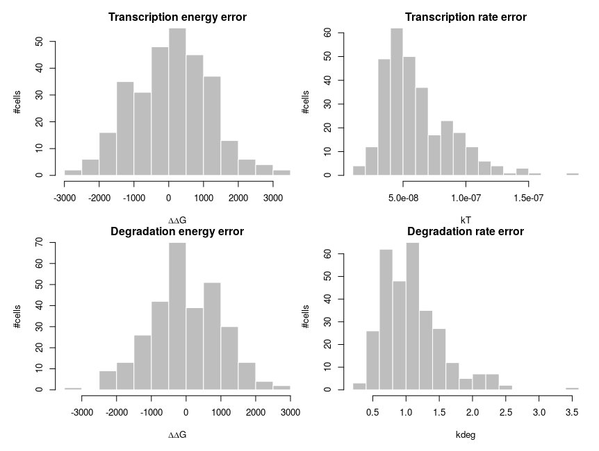
To explain how such asymmetric distributions can arise from noise following normal distributions, we can build a small model of gene expression. mRNA is transcribed at a constant flux, with a rate constant kT. It is then degraded following a unimolecular decay with rate kdeg (chosen to be 1 on average, for convenience). Both rate constants are computed from energies, following the Arrhenius equation, k = Ae-(E/RT), where R is the gas constant, 8.314 and T is the temperature, that we set at 310 K (37 deg C). To simplify we’ll just set the scaling factor A to 1, assuming it is included in the reference energy. E is 0 for degradation, and we modulate the reference transcription energy to control the level of transcript. Both transcription and degradation energy will be affected by normally distributed noises that represent differences between cells (e.g. concentration and state of enzymes). So Ei = E + noise. Because of Arrhenius equation, the normal distributions of energy are transformed into lognormal distributions of rates. Below I plot the distributions of the noises in the cells and the resulting rates.
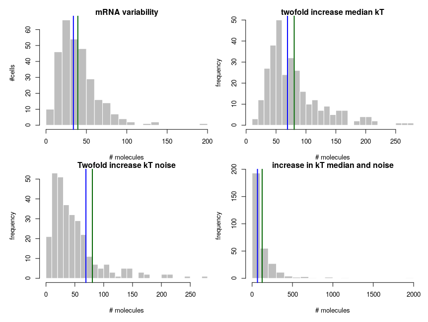
The equilibrium concentration of the mRNA is then kdeg/kT (we could run stochastic simulations to add temporal fluctuations, but that would not change the message). The number of molecules is obtained by multiplying by volume (1e-15 l) and Avogadro number. Each panel presents 300 cells. The distribution on the top-left looks kind of intermediate between those of hexokinase and ACP above. To get the values on the top-right panel, we simulate an overall increase of the transcription rate by twofold, using a decrease of the energy by 8.314*310*ln(2). In this specific case, the observed ratios between the two medians and between the two means are both about 2.04, close to the “truth”. So we could correctly infer a twofold increase by looking at the means. In the bottom panels, we increase the variability of the systems by doubling the standard deviation of the energy noises. Now the ratio of the median is 1.8, inferring a 80% increase while the ratio of the means is 2.53, inferring an increase of 153%!
In summary:
Means of single cell molecular measurements are not a good way of getting a value representing the population;
Comparing the means of single measurements in two populations does not provide an accurate estimation of the underlying changes;
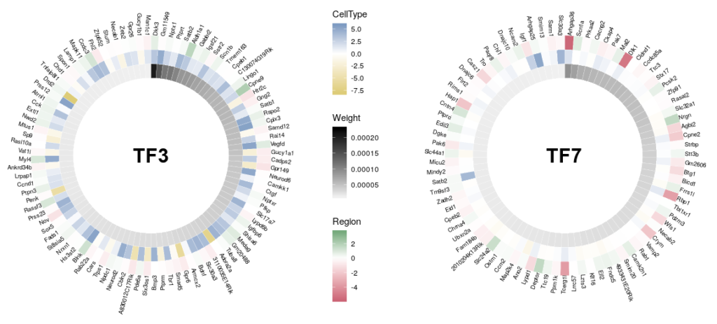
A frequent outcome of network inference based on gene expression data is the discovery of “hubs”, that possibly represent master regulators of our system of interest. Analyzing and comparing those hubs is often at the core of new biological insights. A problem of visualizing network “hubs” is the sheer number of neighbours, that make identification of interesting nodes difficult, and might mask the overall message. The overlay of several features on a nodes, using for instance several colouring or size contributes to the general confusion. Here, we propose to go back from the hub to the wheel, representing each neighbour as a tile in a 360 degree heatmap. In addition, we will used several concentric heatmaps to enable a quick integration of different features. Insight will then come from the comparison of several such wheels.
Of course, tools already exist to represent complex datasets in exquisite circular representations, such as Circos or the R package circlize. But here we will only use ggplot2 and a bit of magic.
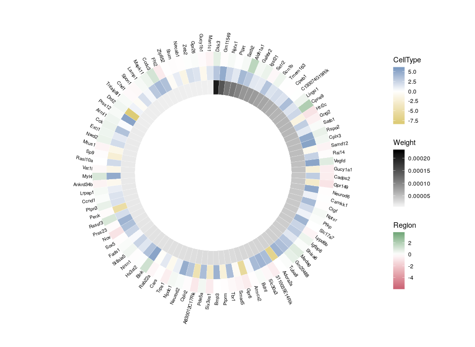
Here is the final figure, showing two transcription factors with their targets, characterised by their expression in cell types, brain regions and the strength of interaction with the hub TFs:
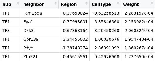
First, we need some data. Using a transcriptomics dataset, we inferred a gene regulatory network (this part of the work is beyond this blog post). The dataset was composed of two cells types coming from two different regions of the brain. For each gene, we computed the log fold difference between regions and between cell types. Our initial edges data table looks like:
TFx are the hub transcription factors that we identified as of interest. neighbor list the top interactors for each hub, weight is a dimensionless factor that represents the significativity of the edge. The higher the more probabl an actual inference exists. The table is ordered by decreasing edge weights.
We will need a few packages.
library(reshape)
library(ggplot2)
library(ggnewscale)   ## The magic
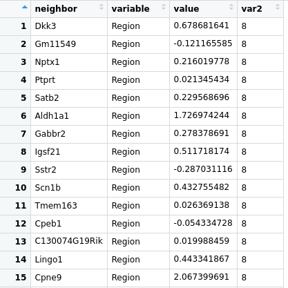
Then we will generate a wheel for a given transcriptions factor (we can, of course, generate a whole bunch of wheels in one go). We extract the information for all its neighbors, and we recast the table using the melt function of the package reshape. We then add an index (var2 below) that will decide where each data will be positioned on the concentric rings..
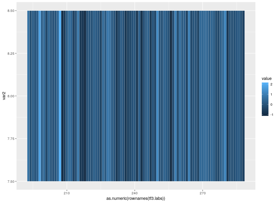
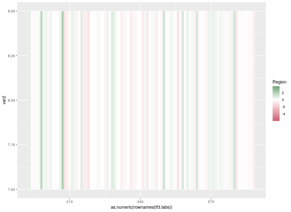
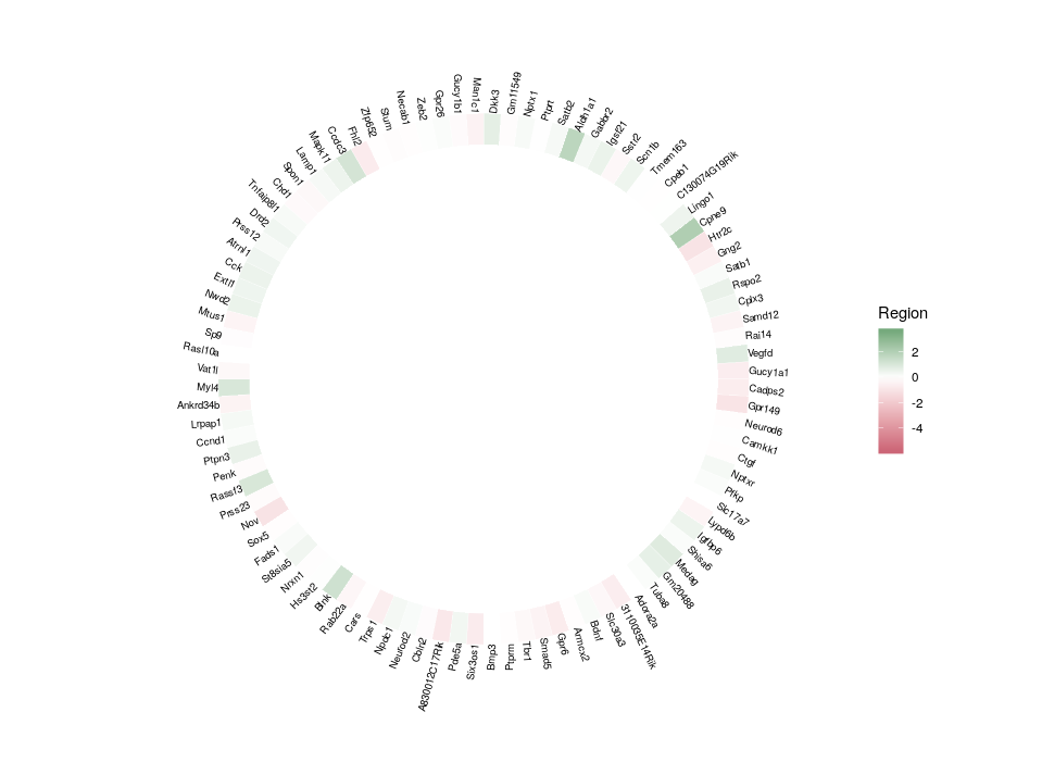
The index starts at 6 so that we have an empty space in the centre corresponding to 5 rings. Now, let’s see the beauty of ggplot2 layered approach in action. We will start with what will be our external ring, the relative expression in different regions.
The default colours are not so nice. Since we want to emphasize the extreme differences of expression, a divergent palette is better suited. Moreover, as we mention above, we want to compare this hub with others. Therefore, the colours must be scaled according to the values across the whole dataset (the initial table edges).
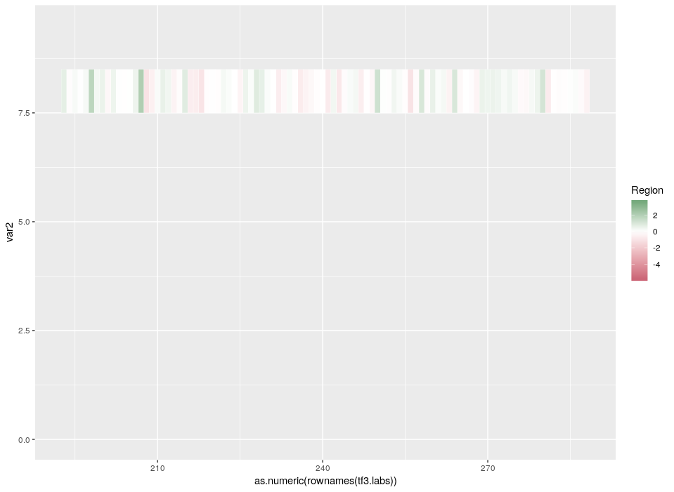
Now, let’s get rid of the useless graphical features that only serve to dilute the main message.
ptf3 <- ptf3 +
  theme(panel.background = element_blank(), # bg of the panel
        panel.grid.major = element_blank(), # get rid of major grid
        panel.grid.minor = element_blank(), # get rid of minor grid
        axis.title=element_blank(),
        panel.grid=element_blank(),
        axis.text.x=element_blank(),
        axis.ticks=element_blank(),
        axis.text.y=element_text(size=0))
plot(ptf3)
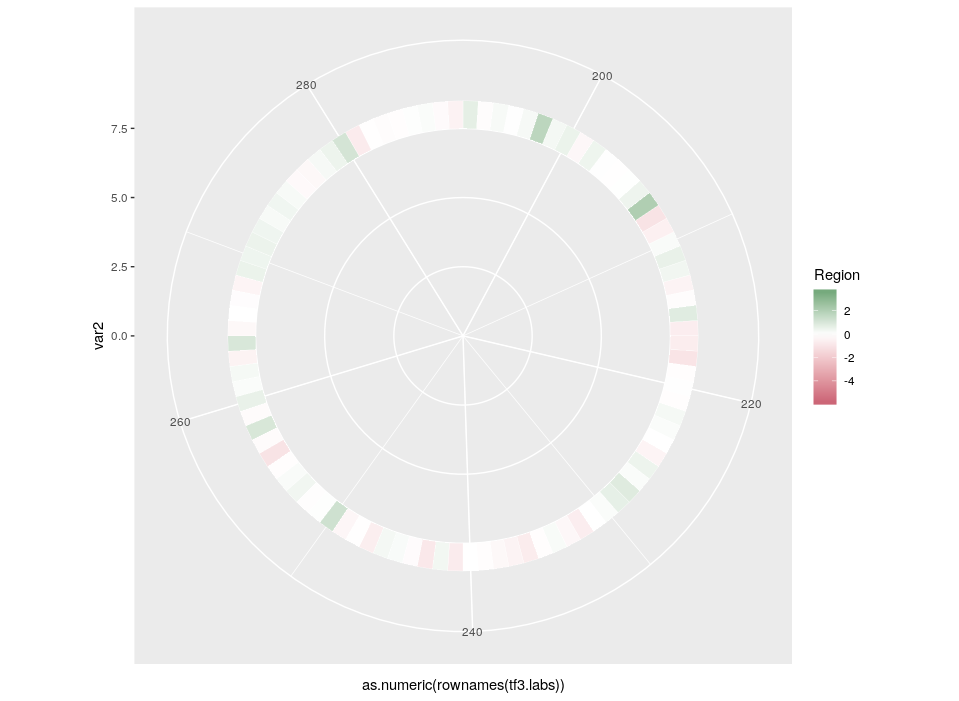
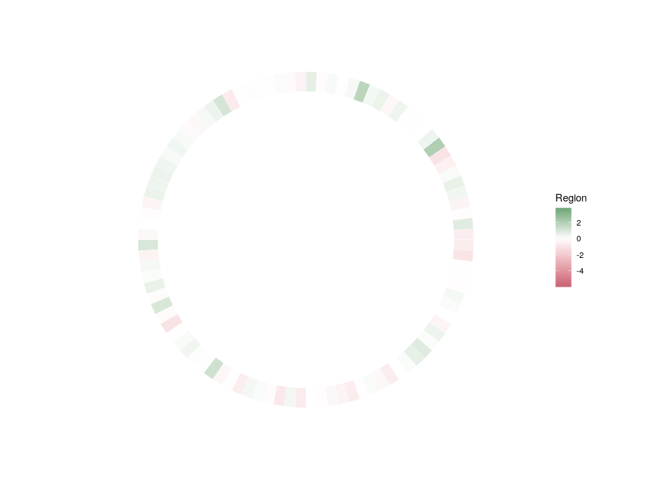
Finally, we can plot the gene names. In order to optimize the readability and use of space, we will plot the names in a radial fashion, but try to make them upright as much as possible. To do so, we need first to compute an angle that depends on the position in the ring. And then, we will compute the required “horizontal” justification, which, when use in conjunction with polar coordinates, produces something quite non-intuitive.
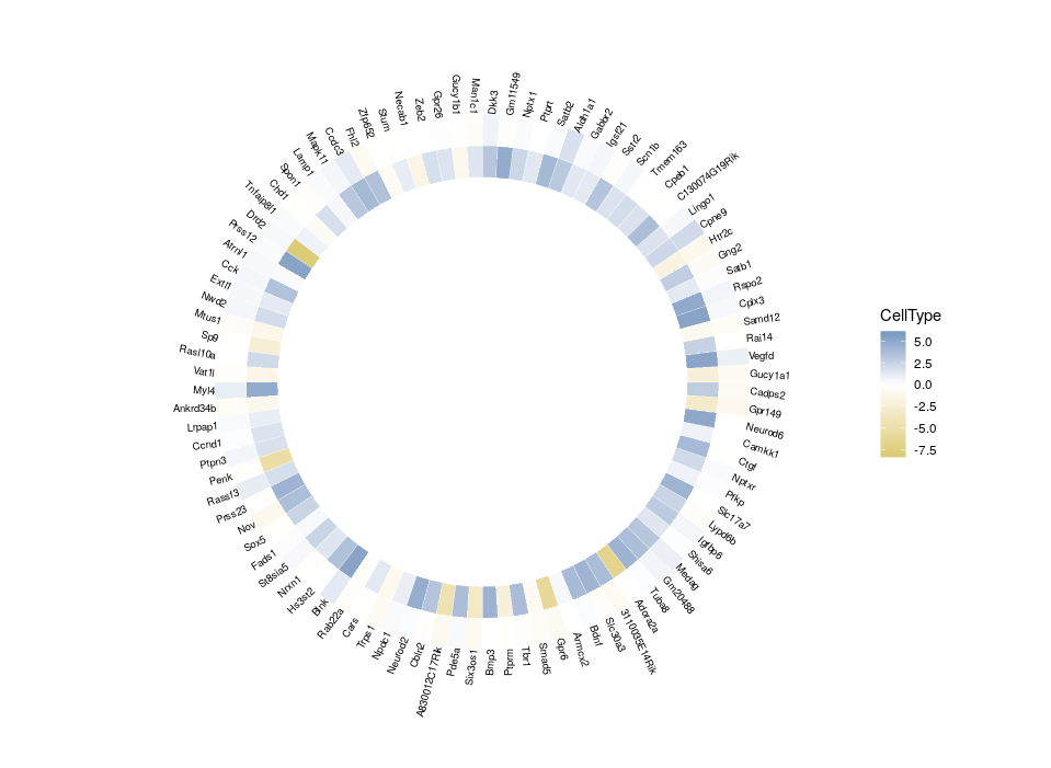
All good. Now that we have plotted the relative expression in different regions, let’s plot the relative expression in different cell types. The first intuitive idea would be to just add a new heatmap inside the previous one. However, since we are talking about a different feature, we want a different colour scale.
Arrgh! First we get an error “Scale for ‘fill’ is already present. Adding another scale for ‘fill’, which will replace the existing scale.” And indeed, the CellType colour scale replaced the Region one for the outer ring. This is because we can only use a single colour scale within a given ggplot2 plot. But not all is lost, thanks to the package ggnewscale which allows us to redefine the colour scale.
NB: Packages like ComplexHeatmap allow to use different colorRamps for different heatmaps. However, they do not allow the use of polar coordinates.
So, here is what we are going to do. We will redefine the scale twice, in order to plot three features on three different concentric heatmaps.
Now we can compare the differential expression of our hub’s neighbours between cell types and between regions. We can do that for several hubs, and compare them, which brings us to our complete figure below. We can see that while the expression of TF3’s neighbours tend to differ strongly between cell types (vivid blues and yellows), they do not differ much between regions (pale greens and magentas). We observe the opposite pattern for TF7, suggesting that TF3 could be regulating spatial-independent cell identity and TF7 could be regulating spatial-dependent cell features.
We are grateful to the following sources that benefited much to this blog post: