By Nicolas Gambardella
Testing is at the core of most, if not all, strategies proposed to fight the Covid-19 pandemic. The “identify and squash” family of approaches relies on identifying cases of people infected by the SARS-CoV-2 virus and isolate and/or treat them. The “get immune” family of approaches relies on identifying people who were infected in the past, and are now immune to the disease, so we can release them. Finally, testing strategies also affect the estimation of how lethal this disease is (see note at the end).
As I write this post (13 April 2020), the UK government just rejected all the blood antibody tests it assessed, the tests that identify people who were in contact with the virus in the past, and supposedly immune. In a similar vein, we can see many reports of “unreliable tests”, catching “only one-third of the cases”. How come professionals designed such “bad” tests? How good a test must be to be useful? And why is a test that correctly spots 90% of infected people not better than the flip of a coin at telling if you are actually infected or not?
There is a short and a long answer. I will give the short one first, so you can stop reading and go back to more enjoyable confinement activities if you so wish.
If we have a test that correctly identifies 90% of the people who were infected (a sensitivity of 90%), and correctly reports as negative 90% of people who were not infected (a specificity of 90%), but at the same time 90% of the whole population was never infected (a prevalence of 10%), and then we test a random sample of this population, we will get the same amount of true and false positive. In other words, if you are tested positive, the chances that you are actually immune is… 50%! You can easily grasp that on the picture below.

The light blue background represents the population that has not been infected while the light pink background represents the population that has been infected (the prevalence). The blue people are tested negative, while the pink people are tested positive. As you can see, we get the same amount of pink people (9) on light pink and light blue backgrounds. Yes, the test comes back positive 9 out of 10 infected people, while it comes back positive only 1 out of 10 non-infected people. But there are 9 non-infected people for each infected one, which tips the balance the other way.
Now, that was just one example, simplified since I assumed equal sensitivity and specificity. For a test detecting the presence of something, sensitivity would typically be lower than specificity (missing something will be more probable than reporting something that is not there). Also, how do the figures change when we change the prevalence, that is the proportion of the population that got infected? Let’s get to the actual calculations.
The basis for such calculus is the Bayes’ theorem, named after the Reverend Thomas Bayes. This post is not about the theorem itself, its meaning or its demonstration. If you are interested to know more, the YouTube channel 3Blue1Brown provides excellent videos on the topic:
The quick proof of Bayes’ theorem
Bayes theorem
For our purpose, you just have to accept the following statement:
Your chances to be actually infected if you tested positive are equal to the chances to be infected in the first place multiplied by the chances of testing positive if actually infected, scaled to the size of the population that tested positive (whether actually infected or not).
In mathematical terms, we would write:
(P(X) means “Probability of X”, the vertical bar “|” represents a conditional probability, the probability that what is on the left side is true given that what is on the right side is true)
P(Infected | Positive) = P(Infected) x P(Positive | Infected) / P(Positive)
This equation, Bayes’ theorem, comes from the fact that:
P(Positive) x P(Infected | Positive) = P(Infected) x P(Positive | Infected)
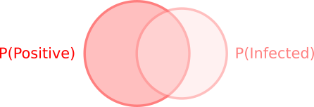
This is obvious from the image below. Whether you draw the left circle first, then the second, or the other way around, the overlapping surface is still the same.
The denominator, P(Positive), representing all people who tested positive, is the sum of the people who rightly tested positive while being infected and the people who wrongly tested positive while not being infected:
P(Positive) = P(Infected) x P(Positive | Infected) + P(NotInfected) x P(Positive | NotInfected)
This probability, P(Infected | Positive), is particularly important in the cases of antibody tests. We do not want to tell a person they are immune if they are not!
Similarly, we can compute the chances that someone who tested negative is actually not infected. That is very important at the beginning of the epidemics when we want to stop infected people to spread the disease.
P(NotInfected | Negative) = P(NotInfected) x P(Negative | NotInfected) / P(Negative)
The denominator, P(Negative), representing all people who tested negative, is the sum of the people who rightly tested negative while not being infected and the people who wrongly tested negative while in fact being infected:
P(Negative) = P(NotInfected) x P(Negative | NotInfected) + P(Infected) x P(Negative | Infected)
Let’s see what we get with actual values. We have three parameters and their complement. Let’s say we have a disease affecting 5% of the population (the prevalence).
P(Infected) = 0.05
P(NotInfected) = 0.95
80% of infected people are caught by the test (its sensitivity).
P(Positive | Infected) = 0.8
P(Negative | Infected) = 0.2
95% of the people who are not infected will not be tested positive (the specificity).
P(Negative | NotInfected) = 0.95
P(Positive | NotInfected) = 0.05.
Now, if you are tested positive, what are the chances you are actually immune?
0.05 x 0.8 / (0.05 x 0.8 + 0.95 x 0.05) = 0.457
46%! In other words, there are 54% chances that you are not actually immune despite being labeled as such by the test… Conversely, if you are tested negative, the chances that you are actually infected are 0.2%. The number looks pretty small, but this can be sufficient to “leak” an infectious patient outside. And this number grows as the prevalence does. How much? The plot below depicts the evolution of probabilities to be correctly tested positive and negative when the proportion of the infected population increases.
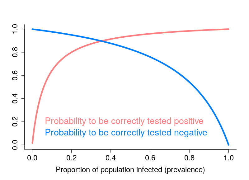
That looks pretty grim, doesn’t it? One way of improving the results is obviously to have better tests. However, the “return on investments” becomes increasingly limited as the quality of tests improves. Another solution, lies in multiple testing, if possible with different tests. This is, for instance, the basis of combined test for Down’s Syndrome. I will let you work out the math if you get twice the same result with two independent tests.
Note about Covid-19’s lethality
Why did I write above that the accuracy of testing was relevant for estimating the lethality of the disease (the Infection Fatality Rate, IFR)? Below is a plot of the ratio number of deaths per number of cases towards the number of tests per million people, for all countries that reported at least 1 death and at least 10 tests (data from 10 April 2020).
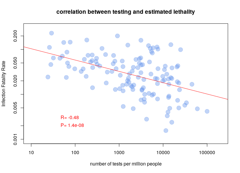
It is pretty clear that there is a correlation, the more tests being done, the lower the estimated fatality. This shows that we probably overestimate the lethality of the disease, and underestimate its prevalence (and therefore its infectiosity). Whether this result is accurate or not, the ability to correctly infer the actual number of people infected and/or immune is pretty crucial. Moreover, the sensitivity and specificity of the tests used by different countries should be taken into account when estimating prevalence and fatality rate.